Opinion

Analyzing the ethical implications and limitations of using artificial intelligence to replace human jobs

In 2005, Ray Kurzweil, a famous futurist, described the Singularity — a point in time when machine intelligence becomes far more powerful than all human intelligence combined. One idea that is closely tied to the Singularity is the automation of human jobs with artificial intelligence.

The automation of human labor is a phenomenon that we can already see today. Cashier-less stores and restaurants with robot servers are just two examples of automation. Some people even believe that at some point, all jobs will be automated by computer programs. But the real question is, can we truly automate all jobs with artificial intelligence? And even if we can automate many jobs, is the world truly ready for full automation?

The Current State of Artificial Intelligence

The first question we have to ask when considering the possibility of an AI-run society is the current state and capability of AI. There are four types of AI, which can be viewed as different levels of sophistication.

1. Reactive AI
2. Limited Memory
3. Theory of Mind
4. Self-Aware

The first two types of AI already exist in today’s world but the last two types are theoretical concepts that will not become a reality until sometime in the future.

Reactive AI

Reactive AI has no concept of memory and is designed to simply react to certain inputs and produce an output. Reactive AI is the simplest form of AI and most early AI systems would fall under this category.

Limited Memory AI

Limited Memory AI is capable of learning from past experience and has a certain degree of memory that allows it to improve its performance over time. Many advances in deep learning such as the use of LSTMs for handling sequential data and the development of reinforcement learning have made this type of AI a reality.

Theory of Mind AI

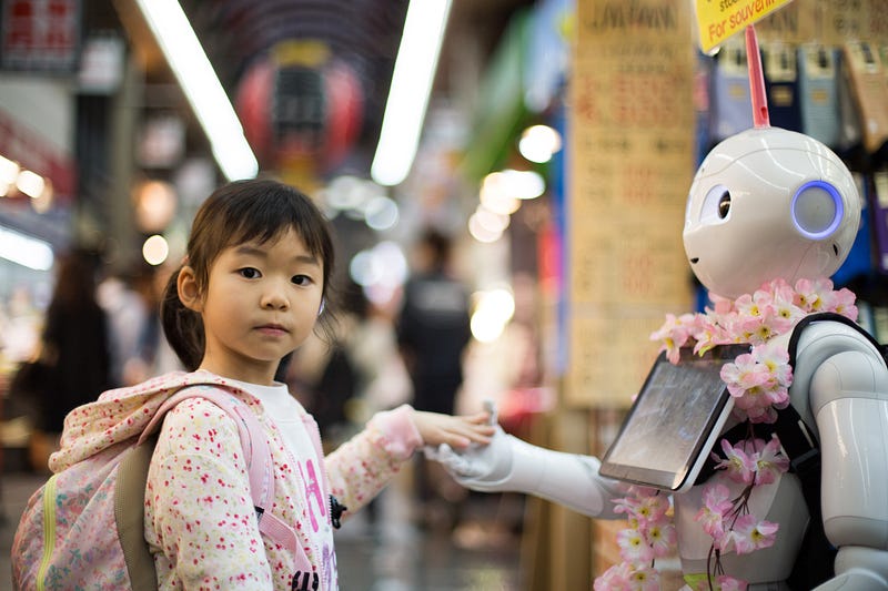
When machines have the ability to interact with the thoughts and feelings of humans, we will have reached “theory of mind” AI. Theory of mind is a concept in psychology that refers to the ability to understand other people by ascribing mental states to them. When machines have this ability, they will have social and emotional intelligence, which enables them to solve a wider range of problems.

Self-Aware AI

Self-aware AI will become a reality when AI enables machines to achieve self-aware intelligence. At this point, machines powered by self-aware AI will be conscious entities, which raises questions about how machines and humans can coexist.

What jobs can easily be automated?

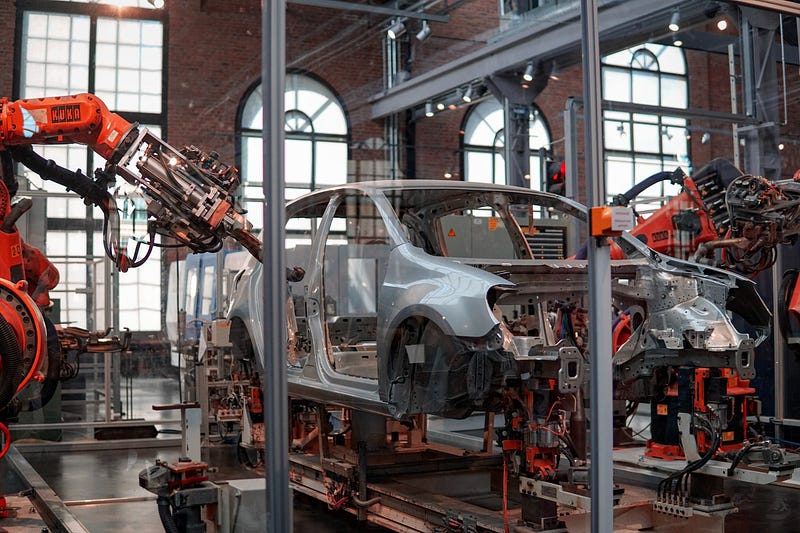
Jobs that involve repetitive steps or predictable decisions can be automated using reactive AI. These jobs often involve manual labor or tasks that involve following clearly defined instructions. Some examples of jobs that fall under this category include:

• Manufacturing and warehouse jobs.
• Manual labor jobs in construction.
• Store clerk and cashier jobs.
• Waste management jobs.
• Manual labor jobs in agriculture (irrigation, harvesting, etc.)

The list above is by no means exhaustive, but the key point here is that all of these jobs involve tasks with clearly defined instructions or predictable decisions that a machine can follow even with reactive AI.

What jobs can eventually be automated?

Jobs that involve more complex decisions based on past events and different situations can eventually be automated but are more difficult to automate than jobs that involve repetitive, algorithmic tasks. A good example of a job that falls under this category is the job of a taxi driver.

There are definitely decision-making patterns that are involved in driving, but drivers need to be able to make situationally-aware decisions. For example, we could train a self-driving car to stop whenever it sees the face of a person. However, what if the car encounters a person whose face is covered? What if the car encounters a dog walking across the road instead of a person? As human beings, we can make these decisions instinctively based on prior experience and what we refer to as “common sense”.

The AI models that power a self-driving car need to be trained to react appropriately to a wide variety of situations and retain some degree of memory regarding past events. In general, jobs that involve more complex, situationally-dependent decision-making can eventually be automated with rigorously trained and tested limited memory AI.

What jobs should be left to humans for now?

Certain jobs require intelligence that is beyond what limited memory AI can provide to machines. Jobs that require social and emotional intelligence will probably not be automated by AI any time soon. In fact, I would argue that these jobs should be left to humans for now. All of the jobs that I have listed below require a certain degree of social and emotional intelligence that exceeds the limits of our current AI systems.

Mental Health Professionals

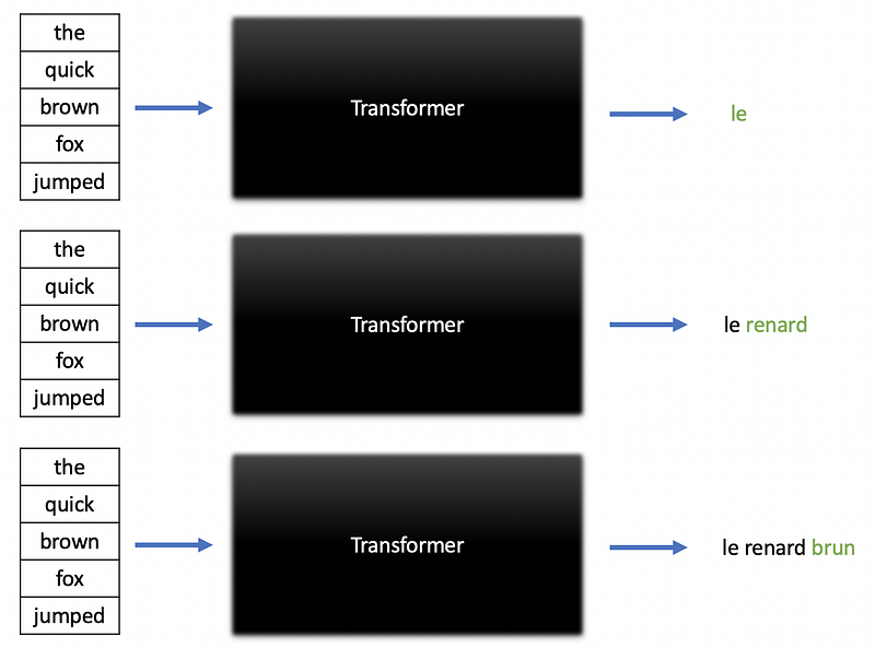
It should come as no surprise that AI, in its current state, cannot effectively automate the jobs of mental health professionals. Therapists, counselors, and psychologists need to be able to understand the emotions and mental states of other people. At the time of writing this article, AI is not capable of understanding human emotions. Some people will argue that large language models such as GPT-3 are capable of human-like conversation, but there is a difference between having a conversation and actually understanding the thoughts and feelings of another person.

Until we achieve Theory of Mind AI, the idea of robot therapists or counselors will not be feasible. In fact, we can rest assured that the jobs of mental health professionals are here to stay for a long time.

Doctors and Medical Personnel

While it may be possible for a machine to perform complex operations such as heart transplants through the use of sophisticated computer vision models, the jobs of doctors and other medical professionals cannot be fully replaced by AI in its current state.

Medical professionals, especially those who work in high-risk environments such as emergency room settings, need to understand the urgency of life and death situations. There are also studies that have shown that empathy is an important part of being a physician. There is a difference between simply curing a disease and actually treating a patient. Treating a patient involves understanding a patient’s concerns and viewing them as a person and not just an illness. A machine driven by limited memory AI can become competent at performing medical procedures, but will always fail to connect with patients on a human level.

There are also ethical concerns that come with using machines to replace the jobs of physicians. For example, if a robot surgeon performs a lung transplant incorrectly and causes serious injury or even death to a patient, then who should be held responsible? Do we blame the doctor who was overseeing the operation? Do we blame programmer behind the robot? Do we blame the robot even though it doesn’t have a conscious mind? These are the types of dilemmas that we will face if we try to automate medical jobs with AI.

Law Enforcement Officers

Like the jobs of mental health professionals and doctors, being a law enforcement officer requires both social and emotional intelligence and a level of situational awareness that surpasses the abilities of even state of the art AI. While it is possible to train a machine to fire a gun or detect a speeding vehicle on the road, limited memory AI is not capable of understanding the urgency of situations where there are threats to the safety of other people. For example, limited memory AI may be capable of tracking down an active shooter in a building but fail to understand that the shooter is putting human lives at risk and causing people in the building to panic.

There are also ethical questions that come with arming machines with firearms and placing the lives of people in a community in the hands of machines with no consciousness. If we arm emotionless machines and make them a part of our police force or the military, what is stopping them from becoming ruthless killing machines? Can a community truly feel comfortable and safe if a large portion of the police force consists of robots? If a machine injures or kills a citizen on duty, who should be held responsible? These questions only highlight the fact that we are not ready for AI to automate law enforcement jobs.

Summary

While AI is indeed a powerful tool that can perform many tasks, we need to understand the limitations of AI, especially when it comes to automating human jobs. The most advanced form of AI that exists today, which includes state-of-the-art models such as GPT-3, is limited-memory AI. Limited-memory AI can learn from past data and experiences but lacks the ability to interact with the thoughts and feelings of humans. This ability, often referred to as theory of mind, is required in a wide range of human jobs.

Without social and emotional intelligence, AI can never truly replace all human jobs. Until theory of mind AI becomes a reality, many essential jobs will still be left to humans.

Join my Mailing List

Join my mailing list to get updates on my data science content. You’ll also get my free Step-By-Step Guide to Solving Machine Learning Problems when you sign up!

And while you’re at it, consider joining the Medium community to read articles from thousands of other writers as well.

Sources

1. A. Hintze, Understanding the four types of AI, from reactive robots to self-aware beings, (2016), The Conversation.
2. L. Greenemeier, 20 Years after Deep Blue: How AI Has Advanced Since Conquering Chess, (2017), Scientific American.
3. E. M., Hirsch, The Role of Empathy in Medicine: A Medical Student’s Perspective, (2007), AMA Journal of Ethics.

How you can use this tree-based algorithm to detect outliers in your data

Anomaly detection is a frequently overlooked area of machine learning. It doesn’t seem anywhere near as flashy as deep learning or natural language processing and often gets skipped entirely in machine learning courses.

However, anomaly detection is still important and has applications ranging from data preprocessing to fraud detection and even system health monitoring. There are many anomaly detection algorithms but the fastest algorithm at the time of writing this article is the Isolation Forest, also known as the iForest.

In this article, I will briefly explain how the Isolation Forest algorithm works and also demonstrate how you can use this algorithm for anomaly detection in Python.

How the Isolation Forest Algorithm Works

The Isolation Forest Algorithm takes advantage of the following properties of anomalous samples (often referred to as outliers):

• Fewness — anomalous samples are a minority and there will only be a few of them in any dataset.
• Different — anomalous samples have values/attributes that are very different from those of normal samples.

These two properties make it easier to isolate anomalous samples from the rest of the data in comparison to normal points.

Notice how in the figure above, we can isolate an anomalous point from the rest of the data with just one line, while the normal point on the right requires four lines to isolate completely.

The Algorithm

Given a sample of data points X, the Isolation Forest algorithm builds an Isolation Tree (iTree), T, using the following steps.

1. Randomly select an attribute q and a split value p.
2. Divide X into two subsets by using the rule q < p. The subsets will correspond to a left subtree and a right subtree in T.
3. Repeat steps 1–2 recursively until either the current node has only one sample or all the values at the current node have the same values.

The algorithm then repeats steps 1–3 multiple times to create several Isolation Trees, producing an Isolation Forest. Based on how Isolation Trees are produced and the properties of anomalous points, we can say that most anomalous points will be located closer to the root of the tree since they are easier to isolate when compared to normal points.

Once we have an Isolation Forest (a collection of Isolation Trees) the algorithm uses the following anomaly score given a data point x and a sample size of m:

In the equation above, h(x) represents the path length of the data point x in a given Isolation Tree. The expression E(h(x)) represents the expected or “average” value of this path length across all the Isolation Trees. The expression c(m) represents the average value of h(x) given a sample size of m and is defined using the following equation.

The equation above is derived from the fact that an Isolation Tree has the same structure as a binary search tree. The termination of a node in an Isolation Tree is similar to an unsuccessful search in a binary search tree as far as the path length is concerned. Once the anomaly score s(x, m) is computed for a given point, we can detect anomalies using the following criteria:

1. If s(x, m) is close to 1 then x is very likely to be an anomaly.
2. If s(x, m) is less than 0.5 then x is likely a normal point.
3. If s(x, m) is close to 0.5 for all of the points in the dataset then the data likely does not contain any anomalies.

Keep in mind that the anomaly score will always be greater than zero but less than 1 for all points so it is quite similar to a probability score.

Using the Isolation Forest Algorithm in Scikit-learn

The Isolation Forest algorithm is available as a module in Scikit-learn. In this tutorial, I will demonstrate how to use Scikit-learn to perform anomaly detection with this algorithm. You can find the full code for this tutorial on GitHub.

Import Libraries

In the code below, I imported some commonly used libraries as well as the Isolation Forest module from Scikit-learn.

import numpy as np
import pandas as pd
from sklearn.ensemble import IsolationForest
import matplotlib.pyplot as plt
%matplotlib inline

Building the Dataset

In order to create a dataset for demonstration purposes, I made use of the make_blobs function from Scikit-learn to create a cluster and added some random outliers in the code below. The entire dataset contains 500 samples and of those 500 samples, only 5 percent or 25 samples are actually anomalies.

from sklearn.datasets import make_blobs

n_samples = 500
outliers_fraction = 0.05
n_outliers = int(outliers_fraction * n_samples)
n_inliers = n_samples - n_outliers

blobs_params = dict(random_state=0, n_samples=n_inliers, n_features=2)

X = make_blobs(centers=[[0, 0], [0, 0]], 
               cluster_std=0.5,
               **blobs_params)[0]

rng = np.random.RandomState(42)

X = np.concatenate([X, rng.uniform(low=-6, high=6, size=(n_outliers, 2))], axis=0)

Training the Algorithm

Training an Isolation Forest is easy to do with Scikit-learn’s API as demonstrated in the code below. Notice that I specified the number of iTrees in the n_estimators argument. There is also another argument named contamination that we can use to specify the percentage of the data that contains anomalies. However, I decided to omit this argument and use the default value because in realistic anomaly detection situations this information will likely be unknown.

iForest = IsolationForest(n_estimators=20, verbose=2)
iForest.fit(X)

Predicting Anomalies

Predicting anomalies is straightforward as demonstrated in the code below.

pred = iForest.predict(X)

The predict function will assign a value of either 1 or -1 to each sample in X. A value of 1 indicates that a point is a normal point while a value of -1 indicates that it is an anomaly.

Visualizing Anomalies

Now that we have some predicted labels for each sample in X, we can visualize the results with Matplotlib as demonstrated in the code below.

plt.scatter(X[:, 0], X[:, 1], c=pred, cmap='RdBu')

The code above produces the visualization below.

In the visualization below, the points that were labeled as anomalies are in red and the normal points are in blue. The algorithm seems to have done a good job at detecting anomalies, although some points at the edge of the cluster in the center may be normal points that were labeled as anomalies instead. Taking a look at the anomaly scores might help us understand the algorithm’s performance a little better.

Visualizing Anomaly Scores

We can generate simplified anomaly scores using the score_samples function as shown below.

pred_scores = -1*iForest.score_samples(X)

Note that the scores returned by the score_samples function will all be negative and correspond to the negative value of the anomaly score defined earlier in this article. For the sake of consistency, I have multiplied these scores by -1.

We can visualize the scores assigned to each point using the code below.

plt.scatter(X[:, 0], X[:, 1], c=pred_scores, cmap='RdBu')
plt.colorbar(label='Simplified Anomaly Score')
plt.show()

The code above gives us the following useful visualization.

When looking at the visualization above, we can see that the algorithm did work as expected since the points that are closer to the blue cluster in the middle have lower anomaly scores, and the points that are further away have higher anomaly scores.

Summary

The Isolation Forest algorithm is a fast tree-based algorithm for anomaly detection. The algorithm uses the concept of path lengths in binary search trees to assign anomaly scores to each point in a dataset. Not only is the algorithm fast and efficient, but it is also widely accessible thanks to Scikit-learn’s implementation.

As usual, you can find the full code for this article on GitHub.

Join my Mailing List

Do you want to get better at data science and machine learning? Do you want to stay up to date with the latest libraries, developments, and research in the data science and machine learning community?

Join my mailing list to get updates on my data science content. You’ll also get my free Step-By-Step Guide to Solving Machine Learning Problems when you sign up!

And while you’re at it, consider joining the Medium community to read articles from thousands of other writers as well.

Sources

1. F. T. Liu, K. M. Ting, and Z. H. Zhou, Isolation Forest, (2008), 2008 Eighth IEEE International Conference on Data Mining.
2. F. Pedregosa et al, Scikit-learn: Machine Learning in Python, (2011), Journal of Machine Learning Research.

An introduction to a more sophisticated approach to topic modeling.

Topic modeling is a problem in natural language processing that has many real-world applications. Being able to discover topics within large sections of text helps us understand text data in greater detail.

For many years, Latent Dirichlet Allocation (LDA) has been the most commonly used algorithm for topic modeling. The algorithm was first introduced in 2003 and treats topics as probability distributions for the occurrence of different words. If you want to see an example of LDA in action, you should check out my article below where I performed LDA on a fake news classification dataset.

https://towardsdatascience.com/fake-news-classification-with-recurrent-convolutional-neural-networks-4a081ff69f1a

However, with the introduction of transformer models and embedding algorithms such as Doc2Vec, we can create much more sophisticated topic models that capture semantic similarities in words. In fact, an algorithm called Top2Vec makes it possible to build topic models using embedding vectors and clustering. In this article, I will demonstrate how you can use Top2Vec to perform unsupervised topic modeling using embedding vectors and clustering techniques.

How does Top2Vec work?

Top2Vec is an algorithm that detects topics present in the text and generates jointly embedded topic, document, and word vectors. At a high level, the algorithm performs the following steps to discover topics in a list of documents.

1. Generate embedding vectors for documents and words.
2. Perform dimensionality reduction on the vectors using an algorithm such as UMAP.
3. Cluster the vectors using a clustering algorithm such as HDBSCAN.
4. Assign topics to each cluster.

I have explained each step in detail below.

Generate embedding vectors for documents and words

An embedding vector is a vector that allows us to represent a word or text document in multi-dimensional space. The idea behind embedding vectors is that similar words or text documents will have similar vectors.

There are many algorithms for generating embedding vectors. Word2Vec and Doc2Vec are quite popular but in recent years, NLP developers and researchers have started using transformers to generate embedding vectors. If you’re interested in learning more about transformers, check out my article below.

https://towardsdatascience.com/fake-news-classification-with-recurrent-convolutional-neural-networks-4a081ff69f1a

Creating embedding vectors for each document allows us to treat each document as a point in multi-dimensional space. Top2Vec also creates jointly embedded word vectors, which allows us to determine topic keywords later.

Once we have a set of word and document vectors, we can move on to the next step.

Perform dimensionality reduction

After we have vectors for each document, the next natural step would be to divide them into clusters using a clustering algorithm. However, the vectors generated from the first step can have as many as 512 components depending on the embedding model that was used.

For this reason, it makes sense to perform some kind of dimensionality reduction algorithm to reduce the number of dimensions in the data. Top2Vec uses an algorithm called UMAP (Uniform Manifold Approximation and Projection) to generate lower-dimensional embedding vectors for each document.

Cluster the vectors

Top2Vec uses HDBSCAN, a hierarchical density-based clustering algorithm, to find dense areas of documents. HDBSCAN is basically just an extension of the DBSCAN algorithm that converts it into a hierarchical clustering algorithm. Using HDBSCAN for topic modeling makes sense because larger topics can consist of several subtopics.

Assign topics to each cluster

Once we have clusters for each document, we can simply treat each cluster of documents as a separate topic in the topic model. Each topic can be represented as a topic vector that is essentially just the centroid (average point) of the original documents belonging to that topic cluster. In order to label the topic using a set of keywords, we can compute the n-closest words to the topic centroid vector.

Once we have keywords for each topic, the algorithm’s job is done, and it’s up to us as humans to interpret what these topics really mean. While Top2Vec is much more complex than the standard LDA approach to topic modeling, it may be able to give us better results since the embedding vectors for words and documents can effectively capture the meaning of words and phrases.

Installing Top2Vec

You can install Top2Vec using pip with the following command:

pip install top2vec

You can also install Top2Vec with additional options as demonstrated in the README document in the Top2Vec GitHub repository.

In order to get Top2Vec installed with the pre-trained universal sentence encoders required to follow along with this tutorial, you should run the following command.

pip install top2vec[sentence_encoders]

Top2Vec tutorial

In this tutorial, I will demonstrate how to use Top2Vec to discover topics in the 20 newsgroups text dataset. This dataset contains roughly 18000 newsgroups posts on 20 topics. You can access the full code for this tutorial on GitHub.

Import Libraries

import numpy as np
import pandas as pd
from top2vec import Top2Vec

Reading the Data

For this tutorial, I will be using the 20 newsgroups text dataset. This dataset contains roughly 18000 newsgroups posts on 20 topics. We can download the dataset through Scikit-learn as demonstrated below.

from sklearn.datasets import fetch_20newsgroups

newsgroups = fetch_20newsgroups(subset='all', remove=('headers', 'footers', 'quotes'))

Training a Top2Vec Model

Training a Top2Vec model is very easy and requires only one line of code as demonstrated below.

from top2vec import Top2Vec

model = Top2Vec(articles_df['content'].values, embedding_model='universal-sentence-encoder')

Note that I used the universal sentence encoder embedding model above. You can use this model if you installed Top2Vec with the sentence encoders option. Otherwise, simply remove this argument and the model will be trained with Doc2Vec embeddings by default.

Viewing the Number of Topics

Once a Top2Vec model has been trained on the data, we can use the model object to get information about the topics that were extracted. For example, we can view the number of topics that were discovered using the get_num_topics function as demonstrated below.

model.get_num_topics()

Running the code above produces the following output.

100

Getting Keywords for each Topic

The Top2Vec model has an attribute called topic_words that is basically just a Numpy array with lists of words for each topic.

model.topic_words

Running the code above in a Jupyter notebook cell produces the following output.

array([['recchi', 'potvin', 'nyr', ..., 'pittsburgh', 'binghamton',
        'pitt'],
       ['diagnosed', 'symptoms', 'diagnosis', ..., 'mfm', 'affected',
        'admitted'],
       ['spacecraft', 'jpl', 'orbiter', ..., 'scientist', 'convention',
        'comet'],
       ...,
       ['liefeld', 'wolverine', 'comics', ..., 'requests', 'tickets',
        'lemieux'],
       ['vice', 'pacific', 'bay', ..., 'projects', 'chapter', 'caps'],
       ['armenians', 'ankara', 'armenian', ..., 'discussed',
        'azerbaijani', 'whom']], dtype='<U15')

If we want to see the words for a specific topic, we can simply index this array as demonstrated below.

model.topic_words[0]

The code above gives us the following list of words for topic 0.

array(['recchi', 'potvin', 'nyr', 'nyi', 'lemieux', 'lindros', 'nhl',
       'phillies', 'defenseman', 'mets', 'ahl', 'jagr', 'bruins',
       'sabres', 'cubs', 'gretzky', 'alomar', 'pitchers', 'pitching',
       'clemens', 'canucks', 'inning', 'henrik', 'innings', 'yankees',
       'oilers', 'utica', 'islanders', 'boswell', 'braves', 'hockey',
       'rangers', 'leafs', 'flyers', 'sox', 'playoffs', 'wpg', 'baseball',
       'dodgers', 'espn', 'goalie', 'fuhr', 'playoff', 'ulf', 'hawks',
       'batting', 'tampa', 'pittsburgh', 'binghamton', 'pitt'],
      dtype='<U15')

As we can see, this topic seems to be mostly about sports, particularly baseball and hockey because we see the names of popular baseball teams along with the last names of hockey players.

Creating Topic Word Clouds

We can easily generate word clouds for topics in order to get a better understanding of the frequency of keywords within a topic.

model.generate_topic_wordcloud(0)

Running the code above produces the word cloud below.

The word cloud above is useful because it lets us visually understand the relative frequency of different words with the topic. We can see that words such as “Phillies” and “Lemieux” appear more often than words such as “playoff” or “Tampa”.

Accessing Topic Vectors

The topic_vectors attribute allows us to access the topic vectors for each topic as demonstrated below.

model.topic_vectors

As we can see in the output below, the topic vectors for a Top2Vec model are stored as a two-dimensional Numpy array where each row corresponds to a specific topic vector.

array([[-9.1372393e-03, -8.8540517e-02, -5.1944017e-02, ...,
         2.0455582e-02, -1.1964893e-01, -1.1116098e-04],
       [-4.0708046e-02, -2.6885601e-02,  2.2835255e-02, ...,
         7.2831921e-02, -6.1708521e-02, -5.2916467e-02],
       [-3.2222651e-02, -4.7691587e-02, -2.9298926e-02, ...,
         4.8001394e-02, -4.6445496e-02, -3.5007432e-02],
       ...,
       [-4.3788709e-02, -6.5007553e-02,  5.3533200e-02, ...,
         2.7984662e-02,  6.5978311e-02, -4.4375043e-02],
       [ 1.2126865e-02, -4.5126071e-03, -4.6988029e-02, ...,
         3.7431438e-02, -1.2432544e-02, -5.3018846e-02],
       [-5.2520853e-02,  4.9585234e-02,  5.9694829e-03, ...,
         4.1887209e-02, -2.1055080e-02, -5.4151181e-02]], dtype=float32)

If we want to access the vector for any topic, for example, we can simply index the Numpy array based on the topic number we are looking for.

Using the Model’s Embedding Function

We can also use the embedding model used by the Top2Vec model to generate document embeddings for any section of text as demonstrated below. Note that this is not possible if you did not specify an embedding model when training the Top2Vec model.

embedding_vector = model.embed(["This is a fake news article."])
embedding_vector.shape

Running the function above produces the following output.

TensorShape([1, 512])

Based on the output above, we can see that the embedding model transformed the text into a 512-dimensional vector in the form of a Python Tensor object.

Searching for Topics Using Keywords

We can search for topics using keywords as demonstrated below. Note that the function returns lists of topic keywords, word scores, topic scores, and topic numbers for each topic that is found from the search.

topic_words, word_scores, topic_scores, topic_nums = model.search_topics(keywords=["politics"], num_topics=3)

We can take a look at the topic words and topic scores to see what topics were returned from the search.

topic_words, topic_scores

The code above produces the following output in Jupyter.

([array(['clinton', 'bush', 'president', 'reagan', 'democratic',
         'republicans', 'elected', 'congress', 'wiretap', 'administration',
         'election', 'johnson', 'politically', 'politicians', 'politics',
         'political', 'executive', 'senate', 'bill', 'constitutional',
         'democracy', 'lib', 'government', 'gov', 'iraq', 'corrupt',
         'convention', 'rockefeller', 'nist', 'ford', 'grant',
         'libertarian', 'nuy', 'govt', 'feds', 'libertarians', 'decades',
         'recall', 'ws', 'bureau', 'bullshit', 'nsa', 'stephanopoulos',
         'weren', 'liar', 'koresh', 'affairs', 'barry', 'conservative',
         'secretary'], dtype='<U15'),
  array(['um', 'ci', 'oo', 'll', 'ye', 'hmm', 'un', 'uh', 'y_', 'wt', 'on',
         'uu', 'actually', 'an', 'eh', 'way', 'des', 'er', 'se', 'not',
         'has', 'huh', 'of', 'ya', 'so', 'it', 'in', 'le', 'upon', 'hm',
         'one', 'is', 'es', 'ne', 'at', 'what', 'no', 'au', 'est', 'shut',
         'mm', 'got', 'dont', 'lo', 'tu', 'en', 'the', 'have', 'am',
         'there'], dtype='<U15'),
  array(['libertarian', 'libertarians', 'govt', 'liberties', 'democracy',
         'democratic', 'government', 'conservative', 'gov', 'republicans',
         'governments', 'liberty', 'constitutional', 'opposed', 'communist',
         'politically', 'advocate', 'citizens', 'premise', 'opposition',
         'patents', 'fascist', 'opposing', 'compromise', 'feds', 'liberal',
         'politicians', 'independent', 'reform', 'johnson', 'philosophy',
         'ron', 'citizen', 'aclu', 'politics', 'frankly', 'xt', 'defend',
         'political', 'regulated', 'militia', 'republic', 'radical',
         'against', 'amendment', 'unified', 'argument', 'revolution',
         'senate', 'obey'], dtype='<U15')],
 array([0.23019153, 0.21416718, 0.19618901]))

We can see that the topics are also ranked by topic score. The topics with the highest similarity scores are shown first in the first list above.

Searching for Documents by Topic

We can easily find documents that belong to specific topics with the search_documents_by_topic function. This function requires both a topic number and the number of documents that we want to retrieve.

model.search_documents_by_topic(0, num_docs=1)

Running the function above produces the following output.

(array(['\nI think this guy is going to be just a little bit disappointed.  Lemieux\ntwo, Tocchet, Mullen, Tippett, and Jagr.  I buzzed my friend because I forgot\nwho had scored Mullen\'s goal.  I said, "Who scored?  Lemieux two, Tocchet,\nTippett, Jagr."  The funny part was I said the "Jagr" part non-chalantly as\nhe was in the process of scoring while I was asking this question!!! :-)\n\nAll in all ABC\'s coverage wasn\'t bad.  On a scale of 1-10, I give it about\nan 8.  How were the games in the Chi/St. Louis/LA area???\n\n\nThat\'s stupid!!!  I\'d complain to the television network!  If I were to even\nsee a Pirates game on instead of a Penguins game at this time of the year, I\nand many other Pittsburghers would surely raise hell!!!\n\n\nTexas is off to a good start, they may pull it out this year.  Whoops!  That\nbelongs in rec.sport.baseball!!!'],
       dtype=object),
 array([0.75086796], dtype=float32),
 array([12405]))

We can see that the article above is definitely about baseball, which matches our interpretation of the first topic.

Reducing the Number of Topics

Sometimes the Top2Vec model will discover many small topics and it is difficult to work with so many different topics. Fortunately, Top2Vec allows us to perform hierarchical topic reduction, which iteratively merges similar topics until we have reached the desired number of topics. We can reduce the number of topics in the model from 100 topics to only 20 topics as demonstrated in the code below.

topic_mapping = model.hierarchical_topic_reduction(num_topics=20)

The topic mapping that the function returns is a nested list that explains which topics have been merged together to form the 20 larger topics.

If we want to look at the original topics within topic 1 we can run the following code in Jupyter.

topic_mapping[1]

The code above produces the following list of merged topic numbers.

[52, 61, 75, 13, 37, 72, 14, 21, 19, 74, 65, 15]

Working with this mapping, however, can be a bit tedious so Top2Vec allows us to access information for the new topics with new attributes. For example, we can access the new topic keywords with the topic_words_reduced attribute.

model.topic_words_reduced[1]

Running the code above gives us the following updated list of keywords for topic 1:

array(['irq', 'mhz', 'processor', 'sgi', 'motherboard', 'risc',
       'processors', 'ati', 'dma', 'scsi', 'cmos', 'powerbook', 'vms',
       'vga', 'cpu', 'packard', 'bsd', 'baud', 'maxtor', 'ansi',
       'hardware', 'ieee', 'xt', 'ibm', 'computer', 'workstation', 'vesa',
       'printers', 'deskjet', 'msdos', 'modems', 'intel', 'printer',
       'linux', 'floppies', 'computing', 'implementations',
       'workstations', 'hp', 'macs', 'monitor', 'vram', 'unix', 'telnet',
       'bios', 'pcs', 'specs', 'oscillator', 'cdrom', 'pc'], dtype='<U15')

Based on the keywords above, we can see that this topic seems to be mostly about computer hardware.

For more details about the functions that are available in Top2Vec, please check out the Top2Vec GitHub repository. I hope you found this tutorial to be useful.

Summary

Top2Vec is a recently developed topic modeling algorithm that may replace LDA in the near future. Unlike LDA, Top2Vec generates jointly embedded word and document vectors and clusters these vectors in order to find topics within text data. The open-source Top2Vec library is also very easy to use and allows developers to train sophisticated topic models in just one line of code.

As usual, you can find the full code for this article on GitHub.

Join my Mailing List

Do you want to get better at data science and machine learning? Do you want to stay up to date with the latest libraries, developments, and research in the data science and machine learning community?

Join my mailing list to get updates on my data science content. You’ll also get my free Step-By-Step Guide to Solving Machine Learning Problems when you sign up!

And while you’re at it, consider joining the Medium community to read articles from thousands of other writers as well.

Sources

1. D. M. Blei, A. Y. Ng, M. I. Jordan, Latent Dirichlet Allocation, (2003), Journal of Machine Learning Research 3.
2. D. Angelov, Top2Vec: Distributed Representations of Topics, (2020), arXiv.org.
3. L. McInnes, J. Healy, and J. Melville, UMAP: Uniform Manifold Approximation and Projection for Dimension Reduction, (2020), arXiv.org.
4. C. Malzer and M. Baum, A Hybrid Approach To Hierarchical Density-based Cluster Selection, (2021), arXiv.org.

An introduction to this modern gradient-boosting library

If you’ve worked as a data scientist, competed in Kaggle competitions, or even browsed data science articles on the internet, there’s a high chance that you’ve heard of XGBoost. Even today, it is often the go-to algorithm for many Kagglers and data scientists working on general machine learning tasks.

While XGBoost is popular for good reasons, it does have some limitations, which I mentioned in my article below.

https://towardsdatascience.com/why-xgboost-cant-solve-all-your-problems-b5003a62d12a

Odds are, you’ve probably heard of XGBoost, but have you ever heard of CatBoost? CatBoost is another open-source gradient boosting library that was created by researchers at Yandex. While it might be slower than XGBoost, it still has several interesting features and could be used as an alternative or included in an ensemble model with XGBoost. For some benchmark datasets, CatBoost has even outperformed XGBoost.

In this article, I will compare this framework to XGBoost and demonstrate how to train a CatBoost model on a simple dataset.

How is CatBoost Different from XGBoost?

Like XGBoost, CatBoost is also a gradient-boosting framework. However, CatBoost has several features, such as the ones listed below, that make it different from XGBoost:

• CatBoost is a different implementation of gradient boosting and makes use of a concept called ordered boosting, which is covered in depth in the CatBoost paper.
• Because CatBoost features a different implementation of gradient boosting, it has the potential to outperform other implementations on certain tasks.
• CatBoost features visualization widgets for cross-validation and grid search that can be viewed in Jupyter notebooks.
• The Pool module in CatBoost supports preprocessing for categorical and text features.

For a complete list of features, be sure to check out the CatBoost documentation page. While CatBoost does have additional features, the main drawback of this implementation is that it is generally slower than XGBoost. But if you are willing to sacrifice speed, this tradeoff may be justifiable in certain situations.

Installation

To install CatBoost with pip, simply run the command listed below.

pip install catboost

Alternatively, you can also install CatBoost with Conda using the following commands.

conda config --add channels conda-forge
conda install catboost

Classification with CatBoost

In this tutorial, I will demonstrate how to train a classification model with CatBoost using a simple dataset generated using Scikit-learn. You can find the full code for this tutorial on GitHub.

Import Libraries

In the code below, I imported basic libraries like Numpy and Pandas along with some modules from CatBoost.

import numpy as np
import pandas as pd
from catboost import CatBoostClassifier, Pool, cv

Creating the Dataset

In the code below, I created a dataset with the make_classification function from Scikit-learn.

from sklearn.datasets import make_classification
X, y = make_classification(n_samples=50000, 
                           n_features=20, 
                           n_informative=15, 
                           n_redundant=5,
                           n_clusters_per_class=5,
                           class_sep=0.7,
                           flip_y=0.03,
                           n_classes=2)

Next, we can split the dataset into training and testing sets using the code below.

from sklearn.model_selection import train_test_split

X_train, X_test, y_train, y_test = train_test_split(X, y, test_size=0.33, random_state=42)

Training the Model

CatBoost has a very simple Scikit-learn style API for training models. We can instantiate a CatBoostClassifier object and train it on the training data as demonstrated in the code below. Note that the iterations argument corresponds to the number of boosting iterations (or the number of trees).

model = CatBoostClassifier(iterations=100,
                           depth=2,
                           learning_rate=1,
                           loss_function='Logloss',
                           verbose=True)

model.fit(X_train, y_train)

Training the model will write the training loss in each iteration to standard output when the verbose argument is set to True.

Note how the total time elapsed, as well as the time remaining is also written to the standard output.

Computing Feature Statistics

We can also compute detailed feature statistics from the training dataset using the calc_feature_statistics function as demonstrated below.

model.calc_feature_statistics(X_train, y_train, feature=1, plot=True)

Note that the feature argument indicates which feature to calculate statistics for. This argument can either be an integer for an index, a string to specify a feature name, or a list of strings or integers to specify multiple features.

The graph above helps us understand the model’s behavior when it comes to predicting targets from feature values in different bins. These bins correspond to different value ranges for the specified feature and are used when creating the decision trees in the CatBoost model.

Getting Feature Importances

We can also compute feature importance with a trained CatBoost model. In order to do this, we first have to take the training data and transform it into a preprocessed CatBoost dataset using the Pool module. After that, we can simply use the get_feature_importance function as demonstrated below.

train_data = Pool(data=X_train, label=y_train)

model.get_feature_importance(train_data)

The function returns a Numpy array of feature importances as shown below.

array([3.01594829, 7.75329451, 5.20064972, 4.43992429, 4.30243392,
       8.32023227, 9.08359773, 2.73403973, 7.11605088, 2.31413571,
       7.76344028, 1.95471762, 6.66177812, 7.78073865, 1.63636954,
       4.66399329, 4.33191962, 1.836554  , 1.96756493, 7.12261691])

Cross-Validation

In order to perform cross-validation with CatBoost, we need to complete the following steps:

1. Create a preprocessed dataset using the Pool module.
2. Create a dictionary of parameters for the CatBoost model.
3. Use the cv function to generate cross-validation scores for the model.

Note that the Pool module also includes optional arguments for preprocessing text and categorical features but since all of the features in our dataset are numerical, I didn’t have to use any of these arguments in this example.

cv_dataset = Pool(data=X_train,
                  label=y_train)

params = {"iterations": 100,
          "depth": 2,
          "loss_function": "Logloss",
          "verbose": False}

scores = cv(cv_dataset,
            params,
            fold_count=5, 
            plot="True")

Running the code above with the plot argument set to True gives us a cool widget shown below in our Jupyter notebook.

On the left-hand side, we can see the cross-validation results for each fold, and on the right-hand side, we can see a graph with the average learning curve for the model along with the standard deviations. The x-axis contains the number of iterations and the y-axis corresponds to the validation loss values.

Grid Search

We can also perform a grid search where the library compares the performance of different hyperparameter combinations to find the best model as demonstrated below.

model = CatBoostClassifier(loss_function='Logloss')

grid = {'learning_rate': [0.03, 0.1],
        'depth': [4, 6, 10]}

grid_search_result = model.grid_search(grid,
                                       X=X_train, 
                                       y=y_train,
                                       cv=3,
                                       plot=True)

Running the code above produces the widget demonstrated in the GIF below.

We can access the best parameters in the grid search by selecting the params attribute.

print(grid_search_result['params'])

The print statement above gives us the best parameters in the grid search, listed below.

{'depth': 10, 'learning_rate': 0.1}

Testing the Model

We can generate predictions from a trained CatBoost model by running the predict function.

model.predict(X_test)

Running the predict function above produces a Numpy array of class labels as shown below.

array([0, 1, 0, ..., 0, 1, 1])

If we want to evaluate the model’s performance on the test data, we can use the score function as demonstrated below.

model.score(X_test, y_test)

Running the function above produced the following output.

0.906

Based on the result above, we can see that the model achieved a testing accuracy of 90.6 percent.

Saving the Model

You can also save a CatBoost in various formats, such as PMML as demonstrated in the code below.

model.save_model(
    "catboost.pmml",
    format="pmml",
    export_parameters={
        'pmml_copyright': 'my copyright (c)',
        'pmml_description': 'test model for BinaryClassification',
        'pmml_model_version': '1'
    }
)

Summary

CatBoost is an updated gradient-boosting framework with additional features that make it worth considering as a potential alternative to XGBoost. It may not be as fast, but it does have useful features and has the potential to outperform XGBoost on certain tasks because it is an improved implementation of gradient boosting.

As usual, you can find the code used in this article on GitHub.

Sources

1. L. Prokhorenkova, G. Gusev, et. al, CatBoost: unbiased boosting with categorical features, (2019), arXiv.org.

Using this Python library to send model training updates.

Imagine this scenario — you’re working on a deep learning project and just started a time-consuming training job on a GPU. Based on your estimates, it will take you about fifteen hours for your job to finish. Obviously, you don’t want to watch your model train for that long. But you still want to know when it finishes training while you’re away from your computer or working on a different task.

Recently, HuggingFace released a Python library called knockknock that allows developers to set up and receive notifications when their models are done training. In this article, I will demonstrate how you can use knockknock to receive model training updates on a wide range of platforms in only a few lines of code!

Installing KnockKnock

You can install knockknock easily with Pip using the command below.

pip install knockknock

Please keep in mind that this library has only been tested for Python 3.6 and later versions. If you have an earlier version of Python, I would suggest upgrading to Python 3.6 or higher if you want to use this library.

Training a Simple Neural Network

For the purpose of demonstrating this library, I will define a function that trains a simple CNN on the classic MNIST Handwritten Digits Dataset. To find the full code for this tutorial, check out this GitHub repository.

Import Libraries

In order to get started, we need to import a few modules from Keras.

from keras.utils.np_utils import to_categorical
from keras.models import Sequential
from keras.layers import Conv2D, MaxPooling2D, Flatten, Dense, Dropout, Activation
from keras.datasets import mnist

Load the Data

To keep this tutorial simple, I loaded the MNIST Dataset using Keras. I performed the following standard preprocessing steps as well in the code below:

1. Added an extra dimension to the 28 x 28-pixel training and testing images.
2. Scaled the training and testing data by 255.
3. Converted the numerical targets to categorical one-hot vectors.

(X_train, y_train), (X_test, y_test) = mnist.load_data()
X_train = X_train.reshape(X_train.shape[0], 28, 28,1) # adds extra dimension
X_test = X_test.reshape(X_test.shape[0], 28, 28, 1) # adds extra dimension
input_shape = (28, 28, 1)

X_train = X_train.astype('float32')
X_test = X_test.astype('float32')
X_train /= 255
X_test /= 255

y_train = to_categorical(y_train)
y_test = to_categorical(y_test)

Training the Model

The function below creates a simple CNN, trains it on the training dataset, and returns accuracy and loss values demonstrating the model’s performance on the test dataset.

https://gist.github.com/AmolMavuduru/6d579c67801276b0f9803b15cf474608

I won’t go into detail about the architecture of the neural network in the code above because the focus of this tutorial is on sending model training notifications. I purposely used a simple neural network for this reason.

Getting Desktop Notifications

Now that we have a function that trains a neural network, we can create another function that trains the model and creates desktop notifications when the function starts and finishes executing.

from knockknock import desktop_sender

@desktop_sender(title="Knockknock Desktop Notifier")
def train_model_desktop_notify(X_train, y_train, X_test, y_test):

    return train_model(X_train, 
                       y_train, 
                       X_test, 
                       y_test)

train_model_desktop_notify(X_train, y_train, X_test, y_test)

On my Mac, running the code above produces a popup notification when the training process starts.

Once the job finishes running, it generates another Desktop notification with the results of the function as shown below.

Getting Email Notifications

We can also set up email notifications with knockknock. In order to do this, you need to set up a separate Gmail account to send the email notifications. You’ll also need to allow less secure apps to access your Gmail account in the security settings.

from knockknock import email_sender

@email_sender(recipient_emails=["amolmavuduru@gmail.com"], 
              sender_email="knockknocknotificationstest@gmail.com")
def train_model_email_notify(X_train, y_train, X_test, y_test):

    return train_model(X_train, 
                       y_train, 
                       X_test, 
                       y_test)

train_model_email_notify(X_train, y_train, X_test, y_test)

Running the code produces the following email notification in Gmail.

When the function finishes running we get another notification email shown below.

Getting Slack Notifications

Finally, if you are part of a Slack team that is working on a machine learning project, you can also set up Slack notifications in a channel when your model finishes running. To do this, you need to create a Slack workspace, add a Slack app to it, and get a Slack webhook URL that you can supply to the slack_sender function decorator. Visit the Slack API page and then follow steps 1–3 in this tutorial to create a webhook.

The code below demonstrates how to create a Slack notification given a webhook URL and a specific channel to post in. Please note that I stored my webhook URL in an environment variable for security reasons.

from knockknock import slack_sender
import os

webhook_url = os.environ['KNOCKKNOCK_WEBHOOK']
@slack_sender(webhook_url=webhook_url, channel="#general")
def train_model_slack_notify(X_train, y_train, X_test, y_test):

    return train_model(X_train, 
                       y_train, 
                       X_test, 
                       y_test)

train_model_slack_notify(X_train, y_train, X_test, y_test)

Running the code above produces the following Slack notifications.

This is a great feature if your data science team has a Slack workspace and wants to monitor your model training jobs.

More Notification Options

With knockknock, we can also send notifications on the following platforms:

• Telegram
• Microsoft Teams
• Text Message
• Discord
• Matrix
• Amazon Chime
• DingTalk
• RocketChat
• WeChat Work

For detailed documentation on how to send notifications on these platforms, be sure to check out the project repository on GitHub.

Summary

Knockknock is a useful tool that lets you keep track of your model training jobs with notifications. You can use it to send notifications on a wide variety of platforms and it is great for keeping track of experiments in data science teams.

As usual, you can find all of the code in this article on GitHub.

Join My Mailing List

Do you want to get better at data science and machine learning? Do you want to stay up to date with the latest libraries, developments, and research in the data science and machine learning community?

Join my mailing list to get updates on my data science content. You’ll also get my free Step-By-Step Guide to Solving Machine Learning Problems when you sign up!

Sources

1. Hugging Face, knockknock Github repository, (2020).

How you can use this powerful API for analyzing articles on the web.

In the Information Age, we have a huge amount of information available to us at our fingertips. The internet is so large that actually estimating its size is a complex task. When it comes to information, our problem is not the absence of information, but rather making sense of the vast amount of information available to us.

What if you could automatically sift through hundreds of web pages and gather the most important points and keywords without having to read everything? This is where TLDR comes into play!

TLDR (too long, didn’t read) is an API that I created for text summarization and analysis. Under the hood, it uses NLTK, a classic Python library for natural language processing. In this article, I will demonstrate how you can use TLDR for your text analysis needs.

Getting Started: TLDR on RapidAPI

TLDR is available on RapidAPI as a freemium API. You can get access to the API by subscribing to it on RapidAPI. If you just want to test out the API, select the Basic plan, which is free as long as you don’t exceed 1000 requests per month. To use the API, create a RapidAPI account, navigate to the pricing page here, and select one of the options listed below.

If you plan to use this API just to follow along with the tutorial in this article, I would recommend choosing the Basic subscription plan. Once you subscribe to the API, you will receive an API key that you include in your request headers to access the API.

Summary of Features

At the time of writing this article, TLDR provides users with the following features:

• Text summarization.
• Keyword extraction.
• Sentiment analysis.

In the future, I will expand this API and add additional features, but these are the basic features that you can use today if you decide to subscribe to the API. In the sections that follow, I will demonstrate how you can make use of the GET requests for each of these features using the Python Requests library. You can find the full code for this tutorial on GitHub.

Summarizing Articles

TLDR makes it easy for users to extract summaries from web articles. Let’s say that we want to extract a five-sentence summary from this CNN article about breakthrough infections after being vaccinated for COVID-19. As demonstrated in the code below, we can use the Python Requests library to call the API and get a summary for this article. Note that I stored my RapidAPI key as an environment variable named TLDR_KEY for security reasons.

import requests
import os

url = "https://tldr-text-analysis.p.rapidapi.com/summarize/"

querystring = {"text":"https://www.cnn.com/2021/04/21/health/two-breakthrough-infections-covid-19/index.html", 
               "max_sentences": "5"}

headers = {
    'x-rapidapi-key': os.environ['TLDR_KEY'],
    'x-rapidapi-host': "tldr-text-analysis.p.rapidapi.com"
    }

response = requests.request("GET", url, headers=headers, params=querystring)

print(response.text)

Running the code above produces the following output.

{"summary":"\"We have characterized bona fide examples of vaccine breakthrough manifesting as clinical symptoms,\" the researchers wrote in their study.Among 417 employees at Rockefeller University who were fully vaccinated with either the Pfizer or Moderna shots, two of them or about .5%, had breakthrough infections later, according to the study published on Wednesday in the New England Journal of Medicine.(CNN)For fully vaccinated people, the risk of still getting Covid-19 -- described as \"breakthrough infections\" -- remains extremely low, a new study out of New York suggests.Experts say that some breakthrough cases of Covid-19 in people who have been fully vaccinated are expected, since no vaccine is 100% effective.The other breakthrough infection was in a healthy 65-year-old woman who received her second dose of the Pfizer vaccine on February 9."}

As expected, TLDR gives us a five-sentence summary for the article that looks pretty convincing. You can also pass in a raw text input instead of a URL directly to the API via the text argument and the API will behave in the same manner.

Keyword Extraction

What if we wanted to extract a list of the top ten keywords in this same CNN article? All we need to do is change the API URL from the previous example and adjust the parameters in the query string as demonstrated below.

import requests
import os

url = "https://tldr-text-analysis.p.rapidapi.com/keywords/"

querystring = {"text":"https://www.cnn.com/2021/04/21/health/two-breakthrough-infections-covid-19/index.html", 
               "n_keywords": "10"}

headers = {
    'x-rapidapi-key': os.environ['TLDR_KEY'],
    'x-rapidapi-host': "tldr-text-analysis.p.rapidapi.com"
    }

response = requests.request("GET", url, headers=headers, params=querystring)

print(response.text)

Running the code above produces the following list of keywords.

[{"keyword":"breakthrough","score":8},{"keyword":"infections","score":8},{"keyword":"people","score":7},{"keyword":"covid","score":7},{"keyword":"vaccine","score":7},{"keyword":"cnn","score":4},{"keyword":"new","score":4},{"keyword":"study","score":4},{"keyword":"coronavirus","score":4},{"keyword":"variants","score":3}]

Notice how the keywords are ranked by frequency scores as well.

Sentiment Analysis

We can also perform sentiment analysis on the same article with the sentiment analysis GET request from the TLDR API as demonstrated in the code below.

import requests
import os

url = "https://tldr-text-analysis.p.rapidapi.com/sentiment_analysis/"

querystring = {"text":"https://www.cnn.com/2021/04/21/health/two-breakthrough-infections-covid-19/index.html"}

headers = {
    'x-rapidapi-key': os.environ['TLDR_KEY'],
    'x-rapidapi-host': "tldr-text-analysis.p.rapidapi.com"
    }

response = requests.request("GET", url, headers=headers, params=querystring)

print(response.text)

Running the code above produces the following JSON output.

{"sentiment":"positive","polarity":0.16429704016913318}

The sentiment field in the output above tells us whether the sentiment of the article is positive, negative, or neutral. The polarity field in the output is a number that can range from -1 to 1 and represents how positive or how negative the sentiment of an article is. As we can see from the output above, the API detected a slightly positive sentiment in the article.

Summary

In this article, I demonstrated how you can use TLDR to perform text summarization, keyword extraction, and sentiment analysis on articles from the web. I plan to expand this API and add additional features in the future. Check out the TLDR API page on RapidAPI for more information and feel free to use this API to build your own NLP applications!

As usual, you can find the code for the examples in this article on GitHub.

Join My Mailing List

Do you want to get better at data science and machine learning? Do you want to stay up to date with the latest libraries, developments, and research in the data science and machine learning community?

Join my mailing list to get updates on my data science content. You’ll also get my free Step-By-Step Guide to Solving Machine Learning Problems when you sign up!

Sources

1. J. Howard, Only 2 ‘breakthrough’ infections among hundreds of fully vaccinated people, new study finds, (2021).

How to deploy your ML models quickly with this API-building tool.

Knowing how to integrate machine learning models into usable applications is an important skill for data scientists. In my previous article linked below, I demonstrated how you can quickly and easily build web apps to showcase your models with Streamlit.

https://towardsdatascience.com/how-you-can-quickly-build-ml-web-apps-with-streamlit-62f423503305

However, what if you want to integrate your machine learning model into a larger software solution instead of a simple standalone web application? What if you are working alongside a software engineer who is building a large application and needs to access your model through a REST API? This exactly where FastAPI comes into play.

FastAPI is a Python web framework that makes it easy for developers to build fast (high-performance), production-ready REST APIs. If you’re a data scientist who works mostly with Python, FastAPI is an excellent tool for deploying your models as REST APIs. In this article, I will demonstrate how you can deploy a spam detection model by building a REST API with FastAPI and running the API in a Docker container.

Training a Spam Detection Model

In this section, I will train a simple spam classification model that determines if a text message is spam. I reused the model training code from my previous article about building web apps with Streamlit so I have included the code below with minimal comments.

I used this Spam Classification Dataset from Kaggle to train a neural network for spam classification. The original dataset is available here as the SMS Spam Collection. You can find the full code for this tutorial on GitHub.

https://gist.github.com/AmolMavuduru/3ec8c42c5ec572380c78761c764215d9

The code above performs the following steps:

1. Reads the spam dataset.
2. Splits the spam dataset into training and testing sets.
3. Creates a text preprocessing and deep learning pipeline for spam classification.
4. Trains the model pipeline on the training set.
5. Evaluates the model pipeline on the testing set.
6. Saves the trained model pipeline.

Building the FastAPI App

In this section, I will demonstrate how to take the trained spam detection model and deploy it as a REST API with FastAPI. The code will be written incrementally in a file called main.py that will run the FastAPI app. Please refer to the following Github repo for the complete code.

Import Libraries

In the code below, I imported the necessary libraries for loading the spam detection model and building the FastAPI app.

import joblib
import re
from sklearn.neural_network import MLPClassifier
from sklearn.feature_extraction.text import TfidfVectorizer
from fastapi import FastAPI

Initializing a FastAPI App Instance

With just one line of code, we can initialize a FastAPI instance as shown below.

app = FastAPI()

This app object is responsible for handling the requests for our REST API for different URIs.

Defining a Simple GET Request

Now that we have a FastAPI app object, we can use it to define the output for a simple get request as demonstrated below.

@app.get('/')
def get_root():

return {'message': 'Welcome to the spam detection API'}

The get request above for the root URL simply returns a JSON output with a welcome message. We can run the FastAPI app using the following command.

uvicorn main:app --reload

The command starts a local Uvicorn server and you should see an output similar to the output shown in the screenshot below.

If you go to the localhost URL http://127.0.0.1.8000 in your browser, you should see a JSON message output as demonstrated below.

I have the JSON Viewer Chrome extension installed, which is why I can see the neat output above, if you don’t have this extension installed, the output in your browser will look more like this.

Now that we know how to define a simple GET request with FastAPI, we can define GET requests to retrieve the spam detection model’s predictions.

Loading the Model and Defining Helper Functions

Before defining the GET request that invokes the spam detection model, we need to first load the model and define functions for preprocessing the text data and returning the model’s predictions.

model = joblib.load('spam_classifier.joblib')

def preprocessor(text):
    text = re.sub('<[^>]*>', '', text) # Effectively removes HTML markup tags
    emoticons = re.findall('(?::|;|=)(?:-)?(?:\)|\(|D|P)', text)
    text = re.sub('[\W]+', ' ', text.lower()) + ' '.join(emoticons).replace('-', '')
    return text

def classify_message(model, message):

    message = preprocessor(message)
    label = model.predict([message])[0]
    spam_prob = model.predict_proba([message])

    return {'label': label, 'spam_probability': spam_prob[0][1]}

The preprocessor function above removes emoticons and unwanted characters from the text input while the classify_message function calls the preprocessor function to clean a text message before using the spam detection model to generate predictions. The classify_message function returns a dictionary, which can conveniently be interpreted as a JSON response.

Defining the Spam Detection GET Request

FastAPI makes it really easy to supply and read variables for GET requests. You can supply the inputs of a machine learning model to a GET request using query parameters or path variables.

Using Query Parameters

For a REST API, query parameters are part of the URL string and are prefixed by a “?”. For example, for the spam detection API we are creating, a GET request could look like this:

127.0.0.1.8000/spam_detection_query/?message=’hello, please reply to this message’

Notice how the message argument at the end is a query parameter. We can write a function that accepts a message as a query parameter and classifies it as ham or spam as demonstrated below.

@app.get('/spam_detection_query/')
async def detect_spam_query(message: str):

   return classify_message(model, message)

If we navigate to the localhost URL, we can test this code with a sample message.

Using Path Variables

When using path variables, the input data is passed to the API as a path in the URL. In this case, a GET request could look like this:

127.0.0.1.8000/spam_detection_query/hello, please reply to this message

Notice how the message is just a part of the URL path and we didn’t have to use any query parameters. We can write a GET request that accepts the message in this format as demonstrated below.

@app.get('/spam_detection_path/{message}')
async def detect_spam_path(message: str):

   return classify_message(model, message)

We can test this new GET request by navigating to the API URL from localhost and shown in the GIF below.

At this point, after writing less than 40 lines of code, we have a functioning REST API for spam detection. Check out the full Fast API app code below.

https://gist.github.com/AmolMavuduru/23bdab9b935d8bd344ff0f972c7141ff

Automatically Generated Documentation

If you navigate to http://127.0.0.1:8000/docs you will find the documentation page for the FastAPI app.

We can also use this documentation page to test each of the GET commands as demonstrated in the GIF below.

The great part about Fast API is that this documentation page was generated automatically. We did not have to write any code or invest hours of time into building it.

Deploying the App on Docker

Now that we have a working API, we can easily deploy it anywhere as a Docker container. If you aren’t familiar with Docker, it is basically a tool that lets you package and run applications in isolated environments called containers.

To run the API as a Docker container, you need to first create a directory called app with all of the code files and a Dockerfile in the parent directory with instructions for running the FastAPI app. To do this, open a text file named “Dockerfile” and add the following lines to it.

FROM tiangolo/uvicorn-gunicorn-fastapi:python3.7

COPY ./app /app

WORKDIR /app

RUN pip install sklearn joblib

Your directory structure should look something like this along with a few extra files from training the spam detection model:

.
├── app
│ └── main.py
└── Dockerfile

The Dockerfile above performs the following tasks:

1. Pulls the FastAPI docker image.
2. Copies the contents of the app directory to the image.
3. Makes the app directory the working directory.
4. Installs necessary dependencies such as Scikit-learn and Joblib.

After creating this file, save it and build the Docker image with the following command.

docker build -t myimage .

Once the image has been built, you can run the Docker container with the following command.

docker run -d --name mycontainer -p 80:80 myimage

Now, you should have a Docker container running on your local machine. If you open your Docker dashboard, you should be able to see the container running as pictured in the screenshot below.

If you hover over the container, you should see a button that says “OPEN IN BROWSER” as shown below.

Click on this button to view the container running in your browser. You should see the output of running the GET command from the root URL below.

We can even test this API by going to the documentation page at localhost/docs.

As demonstrated in the screenshot below, we can easily tell that the API is working as expected, but this time it is running on a Docker container.

Now that the API is running in a Docker container, we can deploy it on a wide range of platforms. If you’re interested in taking this project a step further, check out some of the links below if you want to deploy this API on a cloud platform.

How to Deploy Docker Containers on AWS

Deploy Docker Containers on Azure

Deploy Docker Containers on Google Cloud Platform

Summary

In this article, I demonstrated how you can use FastAPI along with Docker to quickly deploy a spam detection model. FastAPI is a lightweight and fast framework that data scientists can use to create APIs for machine learning models that can easily be integrated into larger applications.

As usual, you can find the code for this article on GitHub.

Join My Mailing List

Do you want to get better at data science and machine learning? Do you want to stay up to date with the latest libraries, developments, and research in the data science and machine learning community?

Join my mailing list to get updates on my data science content. You’ll also get my free Step-By-Step Guide to Solving Machine Learning Problems when you sign up!

Sources

1. S. Ramirez, FastAPI Documentation, (2021).

The quickest way to embed your models into web apps.

If you’re a data scientist or a machine learning engineer, you are probably reasonably confident in your ability to build models to solve real-world business problems. But how good are you at front-end web development? Can you build a visually appealing web application to showcase your models? Chances are, you may be a Python specialist, but not a front-end Javascript expert.

But thankfully, you don’t have to be one! Streamlit is a Python framework that makes it very easy for machine learning and data science practitioners to build web apps in pure Python. That’s right, you don’t even have to worry about HTML tags, Bootstrap components, or writing your own Javascript functions.

In this article, I will demonstrate how you can use Streamlit to quickly build a web app that showcases a text classification model.

Installing Streamlit

You can easily install Streamlit with pip using the command below.

pip install streamlit

Training a Text Classification Model

In this section, I will train a simple spam classification model that determines if a text message is spam. Since the main focus of this tutorial is demonstrating how to use Streamlit, I will include the code used to build this model with minimal comments. I used this Spam Classification Dataset from Kaggle to train a neural network for spam classification. The original dataset is available here as the SMS Spam Collection. You can find the full code for this tutorial on GitHub.

https://gist.github.com/AmolMavuduru/6f9da0a382fd41362da5cf0458bbc7de

The code above performs the following steps:

1. Reads the spam dataset.
2. Splits the spam dataset into training and testing sets.
3. Creates a text preprocessing and deep learning pipeline for spam classification.
4. Trains the model pipeline on the training set.
5. Evaluates the model pipeline on the testing set.
6. Saves the trained model pipeline.

Building a Streamlit App

In the same folder as the saved model pipeline, I created a file called streamlit_app.py and added code incrementally as demonstrated in the sections below. Refer to this GitHub repository if you want to see the full code for this tutorial.

Import Libraries

I imported the necessary libraries and modules, including Streamlit, needed to run this app as shown below.

import joblib
import re
from sklearn.neural_network import MLPClassifier
from sklearn.feature_extraction.text import TfidfVectorizer
import streamlit as st

Creating a Header

Now that we have imported Streamlit, we can quickly create a heading using Streamlit’s Markdown support.

st.write("# Spam Detection Engine")

To see the results of this code, we can run the following command.

streamlit run streamlit_app.py

Running the code and navigating to localhost:8501 gives us the following result.

With just one line of code (not counting the import statements), you now have a running Streamlit app! Next, we can add some interactivity to the app with a text input field.

Adding Text Input

message_text = st.text_input("Enter a message for spam evaluation")

Refreshing the app page at localhost:8501 gives us a neat text input field under the heading.

Now, we can add our trained spam classification model to the app.

Loading the Model

Before loading the model, I included the predefined text preprocessing function since this is a part of the saved model.

def preprocessor(text):
    text = re.sub('<[^>]*>', '', text) 
    emoticons = re.findall('(?::|;|=)(?:-)?(?:\)|\(|D|P)', text)
    text = re.sub('[\W]+', ' ', text.lower()) + ' '.join(emoticons).replace('-', '')
    return text

model = joblib.load('spam_classifier.joblib')

Generating and Displaying Predictions

We can define a special function for returning both the label predicted by the model (spam or ham) and the probability of the message being spam as demonstrated below.

def classify_message(model, message):

  label = model.predict([message])[0]
  spam_prob = model.predict_proba([message])

  return {'label': label, 'spam_probability': spam_prob[0][1]}

Using this function we can output the model’s predictions as a dictionary.

if message_text != '':

  result = classify_message(model, message_text)

  st.write(result)

We can refresh the app again and pass in some sample text inputs. Let’s start with something that is obviously spam.

From the screenshot above, we can see that the model predicts that this message has a very high chance (99.98 percent) of being spam.

Now, let’s write a message about a doctor’s appointment and see if the model classifies it as spam or ham.

As we can see above, the message has a very low probability of being spam based on the predictions generated by the model.

Explaining the Predictions with LIME

We can add some explanations for the predictions generated by the model using LIME, a library for explainable machine learning. For an in-depth tutorial on how to use this library, take a look at my article about explainable machine learning below.

https://towardsdatascience.com/how-to-make-your-machine-learning-models-more-explainable-f20f75928f37

To use LIME and embed a LIME explanation in the web app, add the following import statements to the top of the code.

from lime.lime_text import LimeTextExplainer
import streamlit.components.v1 as components

The components module from Streamlit allows us to embed custom HTML components in the application. We can create a visualization with LIME and display it on a Streamlit app as an HTML component.

Next, we can add the following code at the end of the last if-block to create a button for explaining the model’s predictions.

explain_pred = st.button('Explain Predictions')

The value of the variable explain_pred will be set to True when the button is clicked on once. We can now generate a text explanation with LIME as demonstrated in the code below.

if explain_pred:
  with st.spinner('Generating explanations'):
   class_names = ['ham', 'spam']
   explainer = LimeTextExplainer(class_names=class_names)
   exp = explainer.explain_instance(message_text, 
   model.predict_proba, num_features=10)
   components.html(exp.as_html(), height=800)

Refreshing the app allows us to generate explanations for the model’s predictions as shown in the GIF below. Notice how the LIME TextExplainer allows the user to understand why the model classified the message as spam by highlighting the most important words that the model used in its decision-making process.

At this point, the app is fully functional and can be used to showcase and explain the predictions generated by the spam classification model. Check out the full code for this app below.

https://gist.github.com/AmolMavuduru/4a5e4defee50ae448c7a2c107036584a

Additional Streamlit Capabilities

The app that I created in this article is definitely useful and can serve as a starting point for similar projects, but it only covers a few of the powerful features of Streamlit. Here are some additional features of Streamlit that you should definitely check out:

• Streamlit supports Markdown and Latex commands, allowing you to include equations in a web app.
• Streamlit allows you to display tables and pandas data frames with a single line of code.
• Streamlit allows you to display charts and visualizations from a wide range of libraries including Matplotlib, Bokeh, Pyplot, Pydeck, and even Graphviz.
• Streamlit allows you to easily display points on a map.
• Streamlit also supports embedding image, audio, and video files in your apps.
• Streamlit makes it easy to deploy open-source applications with Streamlit sharing.

To find out more about what Streamlit can do, check out the Streamlit documentation.

Summary

In this article, I demonstrated how you can use Streamlit to build a web app that showcases a simple text classification model in less than 50 lines of code. Streamlit is definitely a powerful, high-level tool that makes web development easy and simple for data scientists. As usual, you can find all the code for this article on GitHub.

Join My Mailing List

Do you want to get better at data science and machine learning? Do you want to stay up to date with the latest libraries, developments, and research in the data science and machine learning community?

Join my mailing list to get updates on my data science content. You’ll also get my free Step-By-Step Guide to Solving Machine Learning Problems when you sign up!

Sources

1. T. A., Almedia and J. M. Gomez Hidalgo, SMS Spam Collection, (2011), Proceedings of the 2011 ACM Symposium on Document Engineering (DOCENG’11).
2. Streamlit Inc., Streamlit Documentation, (2020), streamlit.io.

Getting Started

Train, visualize, evaluate, interpret, and deploy models with minimal code

When we approach supervised machine learning problems, it can be tempting to just see how a random forest or gradient boosting model performs and stop experimenting if we are satisfied with the results. What if you could compare many different models with just one line of code? What if you could reduce each step of the data science process from feature engineering to model deployment to just a few lines of code?

This is exactly where PyCaret comes into play. PyCaret is a high-level, low-code Python library that makes it easy to compare, train, evaluate, tune, and deploy machine learning models with only a few lines of code. At its core, PyCaret is basically just a large wrapper over many data science libraries such as Scikit-learn, Yellowbrick, SHAP, Optuna, and Spacy. Yes, you could use these libraries for the same tasks, but if you don’t want to write a lot of code, PyCaret could save you a lot of time.

In this article, I will demonstrate how you can use PyCaret to quickly and easily build a machine learning project and prepare the final model for deployment.

Installing PyCaret

PyCaret is a large library with a lot of dependencies. I would recommend creating a virtual environment specifically for PyCaret using Conda so that the installation does not impact any of your existing libraries. To create and activate a virtual environment in Conda, run the following commands:

conda create --name pycaret_env python=3.6
conda activate pycaret_env

To install the default, smaller version of PyCaret with only the required dependencies, you can run the following command.

pip install pycaret

To install the full version of PyCaret, you should run the following command instead.

pip install pycaret[full]

Once PyCaret has been installed, deactivate the virtual environment and then add it to Jupyter with the following commands.

conda deactivate
python -m ipykernel install --user --name pycaret_env --display-name "pycaret_env"

Now, after launching a Jupyter Notebook in your browser, you should be able to see the option to change your environment to the one you just created.

Import Libraries

You can find the entire code for this article in this GitHub repository. In the code below, I simply imported Numpy and Pandas for handling the data for this demonstration.

import numpy as np
import pandas as pd

Read the Data

For this example, I used the California Housing Prices Dataset available on Kaggle. In the code below, I read this dataset into a dataframe and displayed the first ten rows of the dataframe.

housing_data = pd.read_csv('./data/housing.csv')
housing_data.head(10)

The output above gives us an idea of what the data looks like. The data contains mostly numerical features with one categorical feature for the proximity of each house to the ocean. The target column that we are trying to predict is the median_house_value column. The entire dataset contains a total of 20,640 observations.

Initialize Experiment

Now that we have the data, we can initialize a PyCaret experiment, which will preprocess the data and enable logging for all of the models that we will train on this dataset.

from pycaret.regression import *

reg_experiment = setup(housing_data, 
                       target = 'median_house_value', 
                       session_id=123, 
                       log_experiment=True, 
                       experiment_name='ca_housing')

As demonstrated in the GIF below, running the code above preprocesses the data and then produces a dataframe with the options for the experiment.

Compare Baseline Models

We can compare different baseline models at once to find the model that achieves the best K-fold cross-validation performance with the compare_models function as shown in the code below. I have excluded XGBoost in the example below for demonstration purposes.

best_model = compare_models(exclude=['xgboost'], fold=5)

The function produces a data frame with the performance statistics for each model and highlights the metrics for the best performing model, which in this case was the CatBoost regressor.

Creating a Model

We can also train a model in just a single line of code with PyCaret. The create_model function simply requires a string corresponding to the type of model that you want to train. You can find a complete list of acceptable strings and the corresponding regression models on the PyCaret documentation page for this function.

catboost = create_model('catboost')

The create_model function produces the dataframe above with cross-validation metrics for the trained CatBoost model.

Hyperparameter Tuning

Now that we have a trained model, we can optimize it even further with hyperparameter tuning. With just one line of code, we can tune the hyperparameters of this model as demonstrated below.

tuned_catboost = tune_model(catboost, n_iter=50, optimize = 'MAE')

The most important results, in this case, the average metrics, are highlighted in yellow.

Visualizing the Model’s Performance

There are many plots that we can create with PyCaret to visualize a model’s performance. PyCaret uses another high-level library called Yellowbrick for building these visualizations.

Residual Plot

The plot_model function will produce a residual plot by default for a regression model as demonstrated below.

plot_model(tuned_catboost)

Prediction Error

We can also visualize the predicted values against the actual target values by creating a prediction error plot.

plot_model(tuned_catboost, plot = 'error')

The plot above is particularly useful because it gives us a visual representation of the R² coefficient for the CatBoost model. In a perfect scenario (R² = 1), where the predicted values exactly matched the actual target values, this plot would simply contain points along the dashed identity line.

Feature Importances

We can also visualize the feature importances for a model as shown below.

plot_model(tuned_catboost, plot = 'feature')

Based on the plot above, we can see that the median_income feature is the most important feature when predicting the price of a house. Since this feature corresponds to the median income in the area in which a house was built, this evaluation makes perfect sense. Houses built in higher-income areas are likely more expensive than those in lower-income areas.

Evaluating the Model Using All Plots

We can also create multiple plots for evaluating a model with the evaluate_model function.

evaluate_model(tuned_catboost)

Interpreting the Model

The interpret_model function is a useful tool for explaining the predictions of a model. This function uses a library for explainable machine learning called SHAP that I covered in the article below.

https://towardsdatascience.com/how-to-make-your-machine-learning-models-more-explainable-f20f75928f37

With just one line of code, we can create a SHAP beeswarm plot for the model.

interpret_model(tuned_catboost)

Based on the plot above, we can see that the median_income field has the greatest impact on the predicted house value.

AutoML

PyCaret also has a function for running automated machine learning (AutoML). We can specify the loss function or metric that we want to optimize and then just let the library take over as demonstrated below.

automl_model = automl(optimize = 'MAE')

In this example, the AutoML model also happens to be a CatBoost regressor, which we can confirm by printing out the model.

print(automl_model)

Running the print statement above produces the following output:

<catboost.core.CatBoostRegressor at 0x7f9f05f4aad0>

Generating Predictions

The predict_model function allows us to generate predictions by either using data from the experiment or new unseen data.

pred_holdouts = predict_model(automl_model)
pred_holdouts.head()

The predict_model function above produces predictions for the holdout datasets used for validating the model during cross-validation. The code also gives us a dataframe with performance statistics for the predictions generated by the AutoML model.

In the output above, the Label column represents the predictions generated by the AutoML model. We can also produce predictions on the entire dataset as demonstrated in the code below.

new_data = housing_data.copy()
new_data.drop(['median_house_value'], axis=1, inplace=True)
predictions = predict_model(automl_model, data=new_data)
predictions.head()

Saving the Model

PyCaret also allows us to save trained models with the save_model function. This function saves the transformation pipeline for the model to a pickle file.

save_model(automl_model, model_name='automl-model')

We can also load the saved AutoML model with the load_model function.

loaded_model = load_model('automl-model')
print(loaded_model)

Printing out the loaded model produces the following output:

Pipeline(memory=None,
         steps=[('dtypes',
                 DataTypes_Auto_infer(categorical_features=[],
                                      display_types=True, features_todrop=[],
                                      id_columns=[], ml_usecase='regression',
                                      numerical_features=[],
                                      target='median_house_value',
                                      time_features=[])),
                ('imputer',
                 Simple_Imputer(categorical_strategy='not_available',
                                fill_value_categorical=None,
                                fill_value_numerical=None,
                                numer...
                ('cluster_all', 'passthrough'),
                ('dummy', Dummify(target='median_house_value')),
                ('fix_perfect', Remove_100(target='median_house_value')),
                ('clean_names', Clean_Colum_Names()),
                ('feature_select', 'passthrough'), ('fix_multi', 'passthrough'),
                ('dfs', 'passthrough'), ('pca', 'passthrough'),
                ['trained_model',
                 <catboost.core.CatBoostRegressor object at 0x7fb750a0aad0>]],
         verbose=False)

As we can see from the output above, PyCaret not only saved the trained model at the end of the pipeline but also the feature engineering and data preprocessing steps at the beginning of the pipeline. Now, we have a production-ready machine learning pipeline in a single file and we don’t have to worry about putting the individual parts of the pipeline together.

Model Deployment

Now that we have a model pipeline that is ready for production, we can also deploy the model to a cloud platform such as AWS with the deploy_model function. Before running this function, you must run the following command to configure your AWS command-line interface if you plan on deploying the model to an S3 bucket:

aws configure

Running the code above will trigger a series of prompts for information like your AWS Secret Access Key that you will need to provide. Once this process is complete, you are ready to deploy the model with the deploy_model function.

deploy_model(automl_model, model_name = 'automl-model-aws', 
             platform='aws',
             authentication = {'bucket' : 'pycaret-ca-housing-model'})

In the code above, I deployed the AutoML model to an S3 bucket named pycaret-ca-housing-model in AWS. From here, you can write an AWS Lambda function that pulls the model from S3 and runs in the cloud. PyCaret also allows you to load the model from S3 using the load_model function.

MLflow UI

Another nice feature of PyCaret is that it can log and track your machine learning experiments with a machine learning lifecycle tool called MLfLow. Running the command below will launch the MLflow user interface in your browser from localhost.

!mlflow ui

In the dashboard above, we can see that MLflow keeps track of the runs for different models for your PyCaret experiments. You can view the performance metrics as well as the running times for each run in your experiment.

Pros and Cons of Using PyCaret

If you’ve read this far, you now have a basic understanding of how to use PyCaret. While PyCaret is a great tool, it comes with its own pros and cons that you should be aware of if you plan to use it for your data science projects.

Pros

• Low-code library.
• Great for simple, standard tasks and general-purpose machine learning.
• Provides support for regression, classification, natural language processing, clustering, anomaly detection, and association rule mining.
• Makes it easy to create and save complex transformation pipelines for models.
• Makes it easy to visualize the performance of your model.

Cons

• As of now, PyCaret is not ideal for text classification because the NLP utilities are limited to topic modeling algorithms.
• PyCaret is not ideal for deep learning and doesn’t use Keras or PyTorch models.
• You can’t perform more complex machine learning tasks such as image classification and text generation with PyCaret (at least with version 2.2.0).
• By using PyCaret, you are sacrificing a certain degree of control for simple and high-level code.

Summary

In this article, I demonstrated how you can use PyCaret to complete all of the steps in a machine learning project ranging from data preprocessing to model deployment. While PyCaret is a useful tool, you should be aware of its pros and cons if you plan to use it for your data science projects. PyCaret is great for general-purpose machine learning with tabular data but as of version 2.2.0, it is not designed for more complex natural language processing, deep learning, and computer vision tasks. But it is still a time-saving tool and who knows, maybe the developers will add support for more complex tasks in the future?

As I mentioned earlier, you can find the full code for this article on GitHub.

Join My Mailing List

Do you want to get better at data science and machine learning? Do you want to stay up to date with the latest libraries, developments, and research in the data science and machine learning community?

Join my mailing list to get updates on my data science content. You’ll also get my free Step-By-Step Guide to Solving Machine Learning Problems when you sign up!

Sources

1. M. Ali, PyCaret: An open-source, low-code machine learning library in Python, (2020), PyCaret.org.
2. S. M. Lundberg, S. Lee, A Unified Approach to Interpreting Model Predictions, (2017), Advances in Neural Information Processing Systems 30 (NIPS 2017).

Understanding the hype behind this language model that generates human-like text

GPT-3 (Generative Pre-trained Transformer 3) is a language model that was created by OpenAI, an artificial intelligence research laboratory in San Francisco. The 175-billion parameter deep learning model is capable of producing human-like text and was trained on large text datasets with hundreds of billions of words.

“I am open to the idea that a worm with 302 neurons is conscious, so I am open to the idea that GPT-3 with 175 billion parameters is conscious too.” — David Chalmers

Since last summer, GPT-3 has made headlines, and entire startups have been created using this tool. However, it’s important to understand the facts behind what GPT-3 really is and how it works rather than getting lost in all of the hype around it and treating it like a black box that can solve any problem.

In this article, I will give you a high-level overview of how GPT-3 works, as well as the strengths and limitations of the model and how you can use it yourself.

How GPT-3 works

At its core, GPT-3 is basically a transformer model. Transformer models are sequence-to-sequence deep learning models that can produce a sequence of text given an input sequence. These models are designed for text generation tasks such as question-answering, text summarization, and machine translation. The image below demonstrates how a transformer model iteratively generates a translation in French given an input sequence in English.

Transformer models operate differently from LSTMs by using multiple units called attention blocks to learn what parts of a text sequence are important to focus on. A single transformer may have several separate attention blocks that each learn separate aspects of language ranging from parts of speech to named entities. For an in-depth overview of how transformers work, you should check out my article below.

https://towardsdatascience.com/what-are-transformers-and-how-can-you-use-them-f7ccd546071a

GPT-3 is the third generation of the GPT language models created by OpenAI. The main difference that sets GPT-3 apart from previous models is its size. GPT-3 contains 175 billion parameters, making it 17 times as large as GPT-2, and about 10 times as Microsoft’s Turing NLG model. Referring to the transformer architecture described in my previous article listed above, GPT-3 has 96 attention blocks that each contain 96 attention heads. In other words, GPT-3 is basically a giant transformer model.

Based on the original paper that introduced this model, GPT-3 was trained using a combination of the following large text datasets:

• Common Crawl
• WebText2
• Books1
• Books2
• Wikipedia Corpus

The final dataset contained a large portion of web pages from the internet, a giant collection of books, and all of Wikipedia. Researchers used this dataset with hundreds of billions of words to train GPT-3 to generate text in English in several other languages.

Why GPT-3 is so powerful

GPT-3 has made headlines since last summer because it can perform a wide variety of natural language tasks and produces human-like text. The tasks that GPT-3 can perform include, but are not limited to:

• Text classification (ie. sentiment analysis)
• Question answering
• Text generation
• Text summarization
• Named-entity recognition
• Language translation

Based on the tasks that GPT-3 can perform, we can think of it as a model that can perform reading comprehension and writing tasks at a near-human level except that it has seen more text than any human will ever read in their lifetime. This is exactly why GPT-3 is so powerful. Entire startups have been created with GPT-3 because we can think of it as a general-purpose swiss army knife for solving a wide variety of problems in natural language processing.

Limitations of GPT-3

While at the time of writing this article GPT-3 is the largest and arguably the most powerful language model, it has its own limitations. In fact, every machine learning model, no matter how powerful, has certain limitations. This concept is something that I explored in great detail in my article about the No Free Lunch Theorem below.

https://towardsdatascience.com/what-are-transformers-and-how-can-you-use-them-f7ccd546071a

Consider some of the limitations of GPT-3 listed below:

• GPT-3 lacks long-term memory — the model does not learn anything from long-term interactions like humans.
• Lack of interpretability — this is a problem that affects extremely large and complex in general. GPT-3 is so large that it is difficult to interpret or explain the output that it produces.
• Limited input size — transformers have a fixed maximum input size and this means that prompts that GPT-3 can deal with cannot be longer than a few sentences.
• Slow inference time — because GPT-3 is so large, it takes more time for the model to produce predictions.
• GPT-3 suffers from bias — all models are only as good as the data that was used to train them and GPT-3 is no exception. This paper, for example, demonstrates that GPT-3 and other large language models contain anti-Muslim bias.

While GPT-3 is powerful, it still has limitations that make it far from being a perfect language model or an example of artificial general intelligence
(AGI).

How you can use GPT-3

Currently, GPT-3 is not open-source and OpenAI decided to instead make the model available through a commercial API that you can find here. This API is in private beta, which means that you will have to fill out the OpenAI API Waitlist Form to join the waitlist to use the API.

OpenAI also has a special program for academic researchers who want to use GPT-3. If you want to use GPT-3 for academic research, you should fill out the Academic Access Application.

While GPT-3 is not open-source or publicly available, its predecessor, GPT-2 is open-source and accessible through Hugging Face’s transformers library. Feel free to check out the documentation for Hugging Face’s GPT-2 implementation if you want to use this smaller, yet still powerful language model instead.

Summary

GPT-3 has received a lot of attention since last summer because it is by far the largest and arguably most powerful language model created at the time of writing this article. However, GPT-3 still suffers from several limitations that make it far from being a perfect language model or an example of AGI. If you would like to use GPT-3 for research or commercial purposes, you can apply to use Open AI’s API which is currently in private beta. Otherwise, you can always work directly with GPT-2 which is publicly available and open-source thanks to HuggingFace’s transformers library.

Join My Mailing List

Do you want to get better at data science and machine learning? Do you want to stay up to date with the latest libraries, developments, and research in the data science and machine learning community?

Join my mailing list to get updates on my data science content. You’ll also get my free Step-By-Step Guide to Solving Machine Learning Problems when you sign up!

Sources

1. T. Brown, B. Mann, N. Ryder, et. al, Language Models are Few-Shot Learners, (2020), arXiv.org.
2. A. Abid, M. Farooqi, and J. Zou, Persistent Anti-Muslim Bias in Large Language Models, (2021), arXiv.org.
3. Wikipedia, Artificial general intelligence, (2021), Wikipedia the Free Encyclopedia.
4. G. Brockman, M. Murati, P. Welinder and OpenAI, OpenAI API, (2020), OpenAI Blog.
5. A. Vaswani, N. Shazeer, et. al, Attention Is All You Need, (2017), 31st Conference on Neural Information Processing Systems.