How you can use this tree-based algorithm to detect outliers in your data

Anomaly detection is a frequently overlooked area of machine learning. It doesn’t seem anywhere near as flashy as deep learning or natural language processing and often gets skipped entirely in machine learning courses.

However, anomaly detection is still important and has applications ranging from data preprocessing to fraud detection and even system health monitoring. There are many anomaly detection algorithms but the fastest algorithm at the time of writing this article is the Isolation Forest, also known as the iForest.

In this article, I will briefly explain how the Isolation Forest algorithm works and also demonstrate how you can use this algorithm for anomaly detection in Python.

How the Isolation Forest Algorithm Works

The Isolation Forest Algorithm takes advantage of the following properties of anomalous samples (often referred to as outliers):

• Fewness — anomalous samples are a minority and there will only be a few of them in any dataset.
• Different — anomalous samples have values/attributes that are very different from those of normal samples.

These two properties make it easier to isolate anomalous samples from the rest of the data in comparison to normal points.

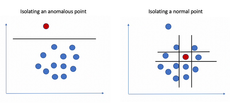
Notice how in the figure above, we can isolate an anomalous point from the rest of the data with just one line, while the normal point on the right requires four lines to isolate completely.

The Algorithm

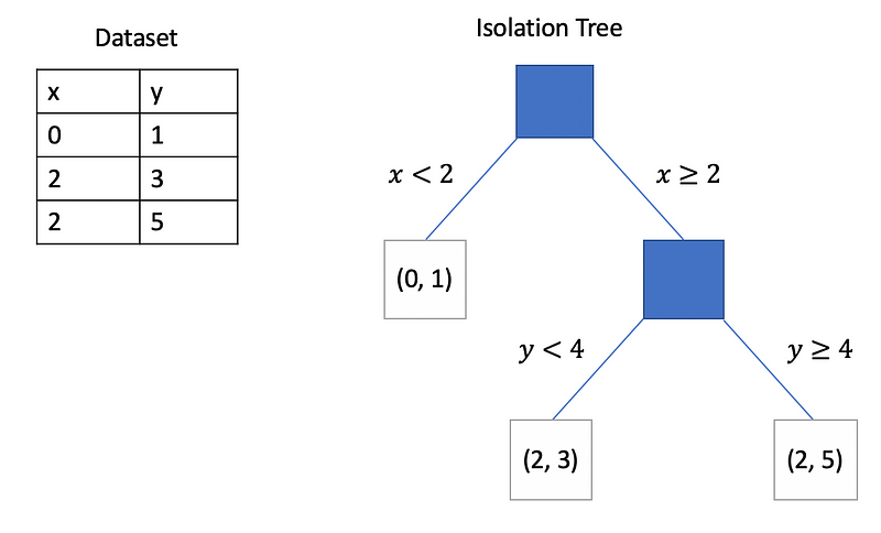
Given a sample of data points X, the Isolation Forest algorithm builds an Isolation Tree (iTree), T, using the following steps.

1. Randomly select an attribute q and a split value p.
2. Divide X into two subsets by using the rule q < p. The subsets will correspond to a left subtree and a right subtree in T.
3. Repeat steps 1–2 recursively until either the current node has only one sample or all the values at the current node have the same values.

The algorithm then repeats steps 1–3 multiple times to create several Isolation Trees, producing an Isolation Forest. Based on how Isolation Trees are produced and the properties of anomalous points, we can say that most anomalous points will be located closer to the root of the tree since they are easier to isolate when compared to normal points.

Once we have an Isolation Forest (a collection of Isolation Trees) the algorithm uses the following anomaly score given a data point x and a sample size of m:

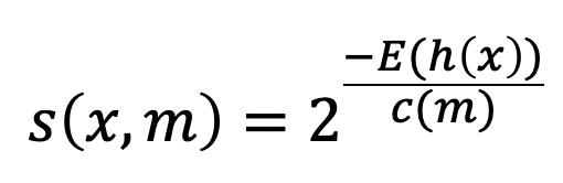
In the equation above, h(x) represents the path length of the data point x in a given Isolation Tree. The expression E(h(x)) represents the expected or “average” value of this path length across all the Isolation Trees. The expression c(m) represents the average value of h(x) given a sample size of m and is defined using the following equation.

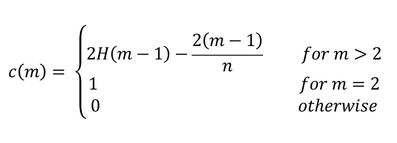
The equation above is derived from the fact that an Isolation Tree has the same structure as a binary search tree. The termination of a node in an Isolation Tree is similar to an unsuccessful search in a binary search tree as far as the path length is concerned. Once the anomaly score s(x, m) is computed for a given point, we can detect anomalies using the following criteria:

1. If s(x, m) is close to 1 then x is very likely to be an anomaly.
2. If s(x, m) is less than 0.5 then x is likely a normal point.
3. If s(x, m) is close to 0.5 for all of the points in the dataset then the data likely does not contain any anomalies.

Keep in mind that the anomaly score will always be greater than zero but less than 1 for all points so it is quite similar to a probability score.

Using the Isolation Forest Algorithm in Scikit-learn

The Isolation Forest algorithm is available as a module in Scikit-learn. In this tutorial, I will demonstrate how to use Scikit-learn to perform anomaly detection with this algorithm. You can find the full code for this tutorial on GitHub.

Import Libraries

In the code below, I imported some commonly used libraries as well as the Isolation Forest module from Scikit-learn.

import numpy as np
import pandas as pd
from sklearn.ensemble import IsolationForest
import matplotlib.pyplot as plt
%matplotlib inline

Building the Dataset

In order to create a dataset for demonstration purposes, I made use of the make_blobs function from Scikit-learn to create a cluster and added some random outliers in the code below. The entire dataset contains 500 samples and of those 500 samples, only 5 percent or 25 samples are actually anomalies.

from sklearn.datasets import make_blobs

n_samples = 500
outliers_fraction = 0.05
n_outliers = int(outliers_fraction * n_samples)
n_inliers = n_samples - n_outliers

blobs_params = dict(random_state=0, n_samples=n_inliers, n_features=2)

X = make_blobs(centers=[[0, 0], [0, 0]], 
               cluster_std=0.5,
               **blobs_params)[0]

rng = np.random.RandomState(42)

X = np.concatenate([X, rng.uniform(low=-6, high=6, size=(n_outliers, 2))], axis=0)

Training the Algorithm

Training an Isolation Forest is easy to do with Scikit-learn’s API as demonstrated in the code below. Notice that I specified the number of iTrees in the n_estimators argument. There is also another argument named contamination that we can use to specify the percentage of the data that contains anomalies. However, I decided to omit this argument and use the default value because in realistic anomaly detection situations this information will likely be unknown.

iForest = IsolationForest(n_estimators=20, verbose=2)
iForest.fit(X)

Predicting Anomalies

Predicting anomalies is straightforward as demonstrated in the code below.

pred = iForest.predict(X)

The predict function will assign a value of either 1 or -1 to each sample in X. A value of 1 indicates that a point is a normal point while a value of -1 indicates that it is an anomaly.

Visualizing Anomalies

Now that we have some predicted labels for each sample in X, we can visualize the results with Matplotlib as demonstrated in the code below.

plt.scatter(X[:, 0], X[:, 1], c=pred, cmap='RdBu')

The code above produces the visualization below.

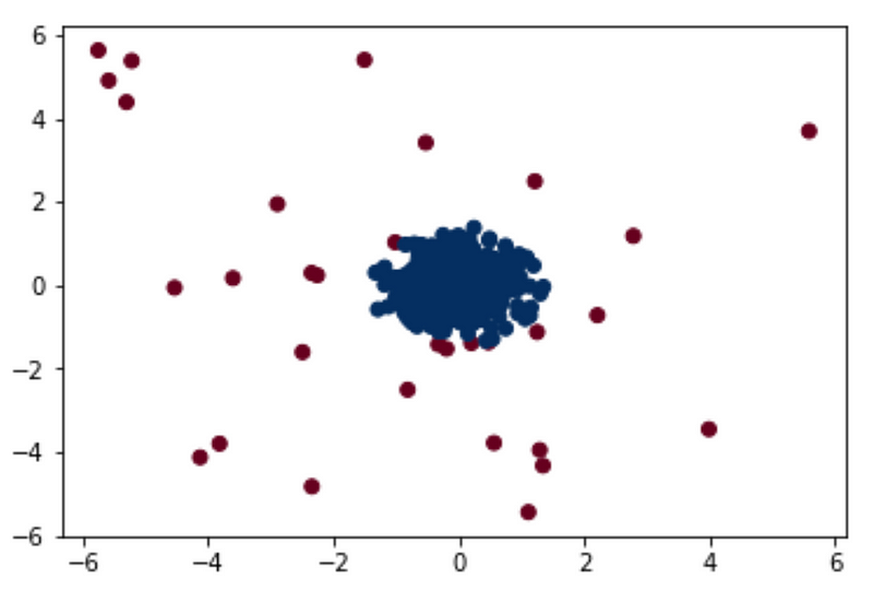
In the visualization below, the points that were labeled as anomalies are in red and the normal points are in blue. The algorithm seems to have done a good job at detecting anomalies, although some points at the edge of the cluster in the center may be normal points that were labeled as anomalies instead. Taking a look at the anomaly scores might help us understand the algorithm’s performance a little better.

Visualizing Anomaly Scores

We can generate simplified anomaly scores using the score_samples function as shown below.

pred_scores = -1*iForest.score_samples(X)

Note that the scores returned by the score_samples function will all be negative and correspond to the negative value of the anomaly score defined earlier in this article. For the sake of consistency, I have multiplied these scores by -1.

We can visualize the scores assigned to each point using the code below.

plt.scatter(X[:, 0], X[:, 1], c=pred_scores, cmap='RdBu')
plt.colorbar(label='Simplified Anomaly Score')
plt.show()

The code above gives us the following useful visualization.

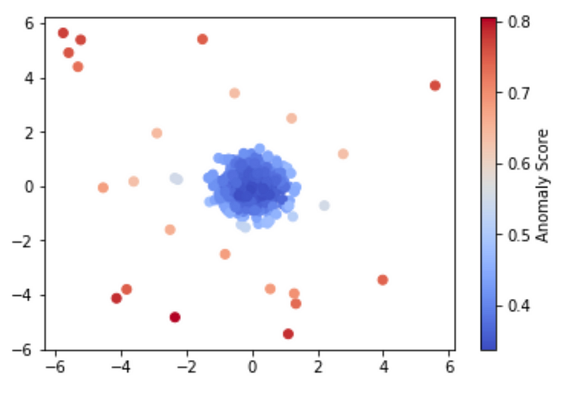
When looking at the visualization above, we can see that the algorithm did work as expected since the points that are closer to the blue cluster in the middle have lower anomaly scores, and the points that are further away have higher anomaly scores.

Summary

The Isolation Forest algorithm is a fast tree-based algorithm for anomaly detection. The algorithm uses the concept of path lengths in binary search trees to assign anomaly scores to each point in a dataset. Not only is the algorithm fast and efficient, but it is also widely accessible thanks to Scikit-learn’s implementation.

As usual, you can find the full code for this article on GitHub.

Join my Mailing List

Do you want to get better at data science and machine learning? Do you want to stay up to date with the latest libraries, developments, and research in the data science and machine learning community?

Join my mailing list to get updates on my data science content. You’ll also get my free Step-By-Step Guide to Solving Machine Learning Problems when you sign up!

And while you’re at it, consider joining the Medium community to read articles from thousands of other writers as well.

Sources

1. F. T. Liu, K. M. Ting, and Z. H. Zhou, Isolation Forest, (2008), 2008 Eighth IEEE International Conference on Data Mining.
2. F. Pedregosa et al, Scikit-learn: Machine Learning in Python, (2011), Journal of Machine Learning Research.