Getting Started

Train, visualize, evaluate, interpret, and deploy models with minimal code

When we approach supervised machine learning problems, it can be tempting to just see how a random forest or gradient boosting model performs and stop experimenting if we are satisfied with the results. What if you could compare many different models with just one line of code? What if you could reduce each step of the data science process from feature engineering to model deployment to just a few lines of code?

This is exactly where PyCaret comes into play. PyCaret is a high-level, low-code Python library that makes it easy to compare, train, evaluate, tune, and deploy machine learning models with only a few lines of code. At its core, PyCaret is basically just a large wrapper over many data science libraries such as Scikit-learn, Yellowbrick, SHAP, Optuna, and Spacy. Yes, you could use these libraries for the same tasks, but if you don’t want to write a lot of code, PyCaret could save you a lot of time.

In this article, I will demonstrate how you can use PyCaret to quickly and easily build a machine learning project and prepare the final model for deployment.

Installing PyCaret

PyCaret is a large library with a lot of dependencies. I would recommend creating a virtual environment specifically for PyCaret using Conda so that the installation does not impact any of your existing libraries. To create and activate a virtual environment in Conda, run the following commands:

conda create --name pycaret_env python=3.6
conda activate pycaret_env

To install the default, smaller version of PyCaret with only the required dependencies, you can run the following command.

pip install pycaret

To install the full version of PyCaret, you should run the following command instead.

pip install pycaret[full]

Once PyCaret has been installed, deactivate the virtual environment and then add it to Jupyter with the following commands.

conda deactivate
python -m ipykernel install --user --name pycaret_env --display-name "pycaret_env"

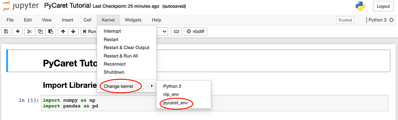
Now, after launching a Jupyter Notebook in your browser, you should be able to see the option to change your environment to the one you just created.

Import Libraries

You can find the entire code for this article in this GitHub repository. In the code below, I simply imported Numpy and Pandas for handling the data for this demonstration.

import numpy as np
import pandas as pd

Read the Data

For this example, I used the California Housing Prices Dataset available on Kaggle. In the code below, I read this dataset into a dataframe and displayed the first ten rows of the dataframe.

housing_data = pd.read_csv('./data/housing.csv')
housing_data.head(10)

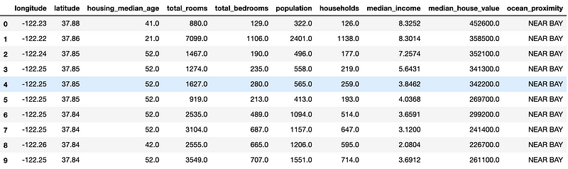
The output above gives us an idea of what the data looks like. The data contains mostly numerical features with one categorical feature for the proximity of each house to the ocean. The target column that we are trying to predict is the median_house_value column. The entire dataset contains a total of 20,640 observations.

Initialize Experiment

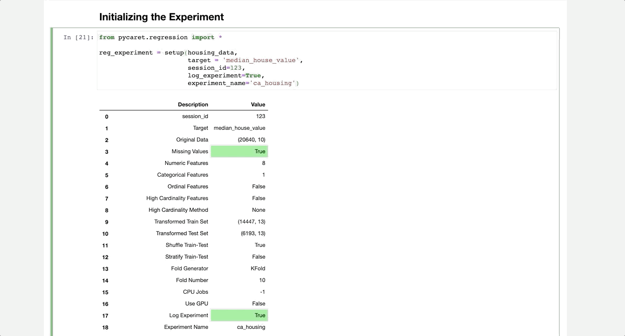
Now that we have the data, we can initialize a PyCaret experiment, which will preprocess the data and enable logging for all of the models that we will train on this dataset.

from pycaret.regression import *

reg_experiment = setup(housing_data, 
                       target = 'median_house_value', 
                       session_id=123, 
                       log_experiment=True, 
                       experiment_name='ca_housing')

As demonstrated in the GIF below, running the code above preprocesses the data and then produces a dataframe with the options for the experiment.

Compare Baseline Models

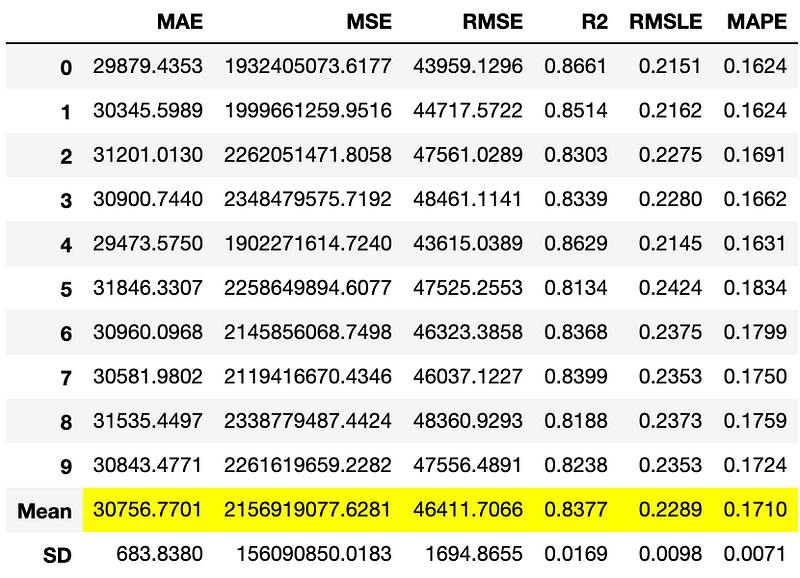
We can compare different baseline models at once to find the model that achieves the best K-fold cross-validation performance with the compare_models function as shown in the code below. I have excluded XGBoost in the example below for demonstration purposes.

best_model = compare_models(exclude=['xgboost'], fold=5)

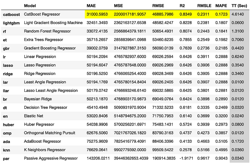
The function produces a data frame with the performance statistics for each model and highlights the metrics for the best performing model, which in this case was the CatBoost regressor.

Creating a Model

We can also train a model in just a single line of code with PyCaret. The create_model function simply requires a string corresponding to the type of model that you want to train. You can find a complete list of acceptable strings and the corresponding regression models on the PyCaret documentation page for this function.

catboost = create_model('catboost')

The create_model function produces the dataframe above with cross-validation metrics for the trained CatBoost model.

Hyperparameter Tuning

Now that we have a trained model, we can optimize it even further with hyperparameter tuning. With just one line of code, we can tune the hyperparameters of this model as demonstrated below.

tuned_catboost = tune_model(catboost, n_iter=50, optimize = 'MAE')

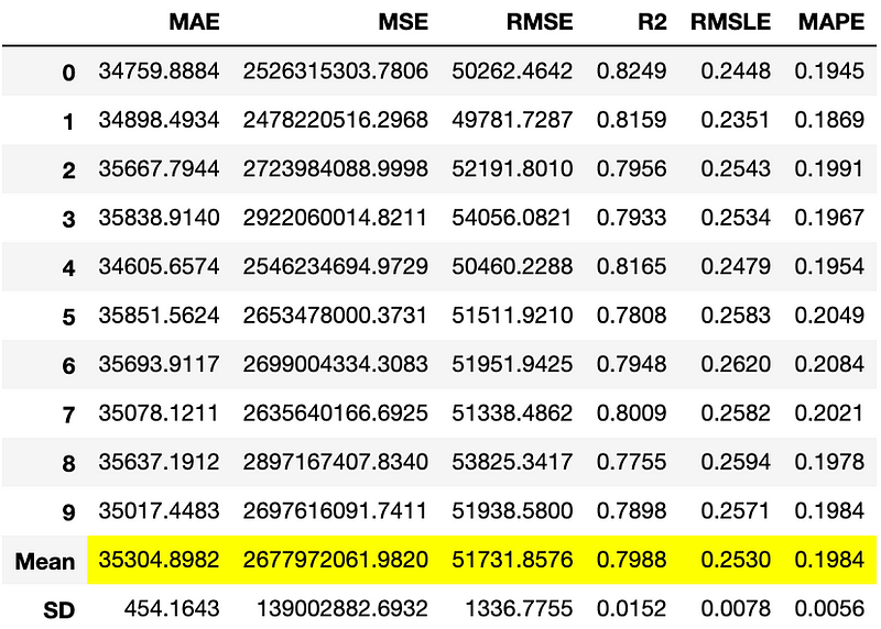
The most important results, in this case, the average metrics, are highlighted in yellow.

Visualizing the Model’s Performance

There are many plots that we can create with PyCaret to visualize a model’s performance. PyCaret uses another high-level library called Yellowbrick for building these visualizations.

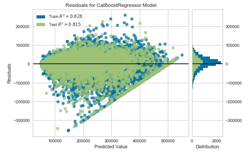
Residual Plot

The plot_model function will produce a residual plot by default for a regression model as demonstrated below.

plot_model(tuned_catboost)

Prediction Error

We can also visualize the predicted values against the actual target values by creating a prediction error plot.

plot_model(tuned_catboost, plot = 'error')

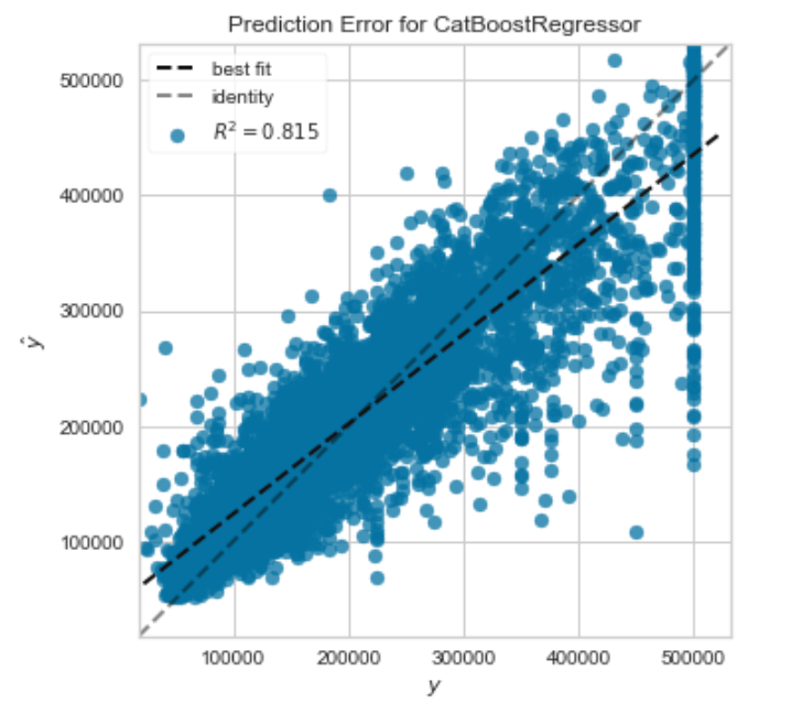
The plot above is particularly useful because it gives us a visual representation of the R² coefficient for the CatBoost model. In a perfect scenario (R² = 1), where the predicted values exactly matched the actual target values, this plot would simply contain points along the dashed identity line.

Feature Importances

We can also visualize the feature importances for a model as shown below.

plot_model(tuned_catboost, plot = 'feature')

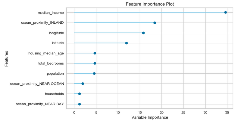
Based on the plot above, we can see that the median_income feature is the most important feature when predicting the price of a house. Since this feature corresponds to the median income in the area in which a house was built, this evaluation makes perfect sense. Houses built in higher-income areas are likely more expensive than those in lower-income areas.

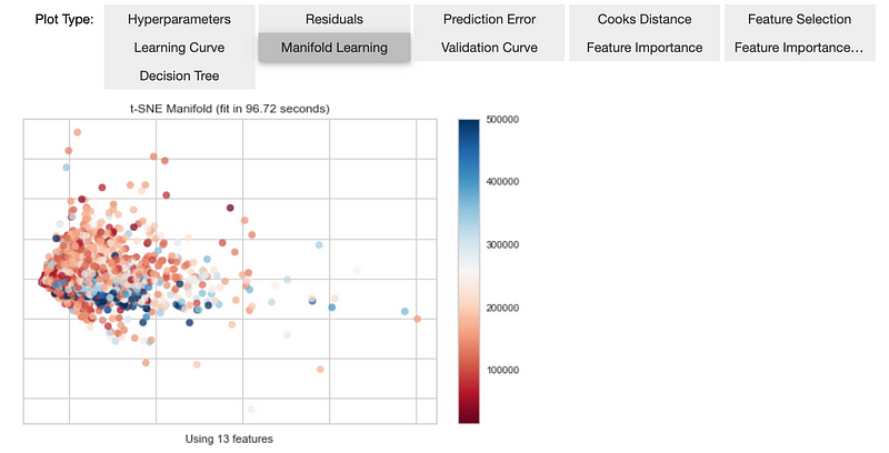
Evaluating the Model Using All Plots

We can also create multiple plots for evaluating a model with the evaluate_model function.

evaluate_model(tuned_catboost)

Interpreting the Model

The interpret_model function is a useful tool for explaining the predictions of a model. This function uses a library for explainable machine learning called SHAP that I covered in the article below.

https://towardsdatascience.com/how-to-make-your-machine-learning-models-more-explainable-f20f75928f37

With just one line of code, we can create a SHAP beeswarm plot for the model.

interpret_model(tuned_catboost)

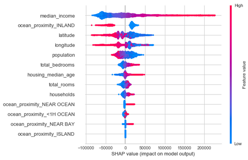
Based on the plot above, we can see that the median_income field has the greatest impact on the predicted house value.

AutoML

PyCaret also has a function for running automated machine learning (AutoML). We can specify the loss function or metric that we want to optimize and then just let the library take over as demonstrated below.

automl_model = automl(optimize = 'MAE')

In this example, the AutoML model also happens to be a CatBoost regressor, which we can confirm by printing out the model.

print(automl_model)

Running the print statement above produces the following output:

<catboost.core.CatBoostRegressor at 0x7f9f05f4aad0>

Generating Predictions

The predict_model function allows us to generate predictions by either using data from the experiment or new unseen data.

pred_holdouts = predict_model(automl_model)
pred_holdouts.head()

The predict_model function above produces predictions for the holdout datasets used for validating the model during cross-validation. The code also gives us a dataframe with performance statistics for the predictions generated by the AutoML model.

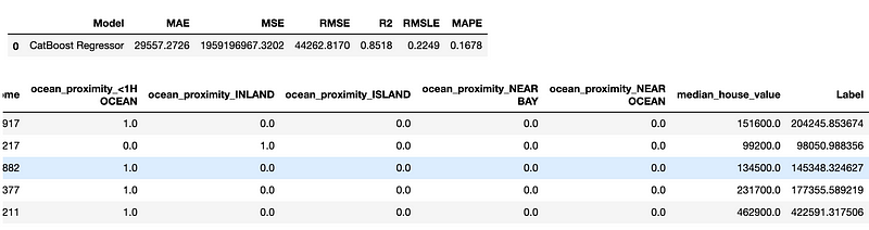
In the output above, the Label column represents the predictions generated by the AutoML model. We can also produce predictions on the entire dataset as demonstrated in the code below.

new_data = housing_data.copy()
new_data.drop(['median_house_value'], axis=1, inplace=True)
predictions = predict_model(automl_model, data=new_data)
predictions.head()

Saving the Model

PyCaret also allows us to save trained models with the save_model function. This function saves the transformation pipeline for the model to a pickle file.

save_model(automl_model, model_name='automl-model')

We can also load the saved AutoML model with the load_model function.

loaded_model = load_model('automl-model')
print(loaded_model)

Printing out the loaded model produces the following output:

Pipeline(memory=None,
         steps=[('dtypes',
                 DataTypes_Auto_infer(categorical_features=[],
                                      display_types=True, features_todrop=[],
                                      id_columns=[], ml_usecase='regression',
                                      numerical_features=[],
                                      target='median_house_value',
                                      time_features=[])),
                ('imputer',
                 Simple_Imputer(categorical_strategy='not_available',
                                fill_value_categorical=None,
                                fill_value_numerical=None,
                                numer...
                ('cluster_all', 'passthrough'),
                ('dummy', Dummify(target='median_house_value')),
                ('fix_perfect', Remove_100(target='median_house_value')),
                ('clean_names', Clean_Colum_Names()),
                ('feature_select', 'passthrough'), ('fix_multi', 'passthrough'),
                ('dfs', 'passthrough'), ('pca', 'passthrough'),
                ['trained_model',
                 <catboost.core.CatBoostRegressor object at 0x7fb750a0aad0>]],
         verbose=False)

As we can see from the output above, PyCaret not only saved the trained model at the end of the pipeline but also the feature engineering and data preprocessing steps at the beginning of the pipeline. Now, we have a production-ready machine learning pipeline in a single file and we don’t have to worry about putting the individual parts of the pipeline together.

Model Deployment

Now that we have a model pipeline that is ready for production, we can also deploy the model to a cloud platform such as AWS with the deploy_model function. Before running this function, you must run the following command to configure your AWS command-line interface if you plan on deploying the model to an S3 bucket:

aws configure

Running the code above will trigger a series of prompts for information like your AWS Secret Access Key that you will need to provide. Once this process is complete, you are ready to deploy the model with the deploy_model function.

deploy_model(automl_model, model_name = 'automl-model-aws', 
             platform='aws',
             authentication = {'bucket' : 'pycaret-ca-housing-model'})

In the code above, I deployed the AutoML model to an S3 bucket named pycaret-ca-housing-model in AWS. From here, you can write an AWS Lambda function that pulls the model from S3 and runs in the cloud. PyCaret also allows you to load the model from S3 using the load_model function.

MLflow UI

Another nice feature of PyCaret is that it can log and track your machine learning experiments with a machine learning lifecycle tool called MLfLow. Running the command below will launch the MLflow user interface in your browser from localhost.

!mlflow ui

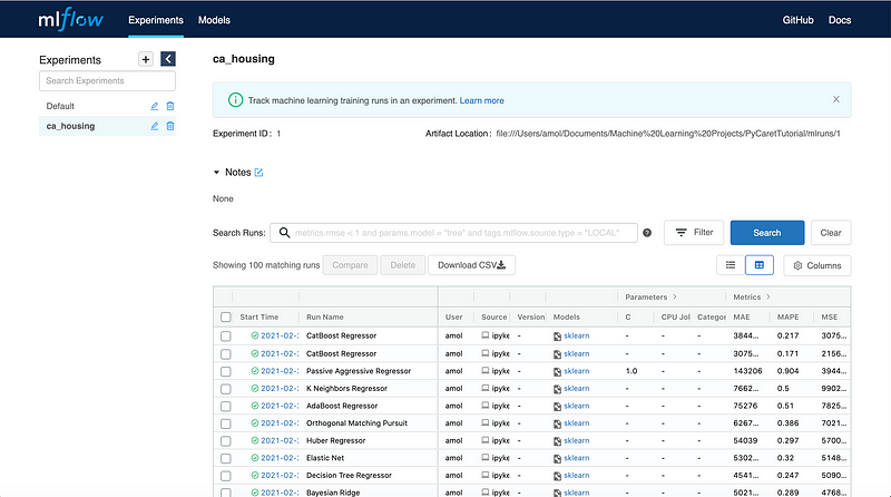
In the dashboard above, we can see that MLflow keeps track of the runs for different models for your PyCaret experiments. You can view the performance metrics as well as the running times for each run in your experiment.

Pros and Cons of Using PyCaret

If you’ve read this far, you now have a basic understanding of how to use PyCaret. While PyCaret is a great tool, it comes with its own pros and cons that you should be aware of if you plan to use it for your data science projects.

Pros

• Low-code library.
• Great for simple, standard tasks and general-purpose machine learning.
• Provides support for regression, classification, natural language processing, clustering, anomaly detection, and association rule mining.
• Makes it easy to create and save complex transformation pipelines for models.
• Makes it easy to visualize the performance of your model.

Cons

• As of now, PyCaret is not ideal for text classification because the NLP utilities are limited to topic modeling algorithms.
• PyCaret is not ideal for deep learning and doesn’t use Keras or PyTorch models.
• You can’t perform more complex machine learning tasks such as image classification and text generation with PyCaret (at least with version 2.2.0).
• By using PyCaret, you are sacrificing a certain degree of control for simple and high-level code.

Summary

In this article, I demonstrated how you can use PyCaret to complete all of the steps in a machine learning project ranging from data preprocessing to model deployment. While PyCaret is a useful tool, you should be aware of its pros and cons if you plan to use it for your data science projects. PyCaret is great for general-purpose machine learning with tabular data but as of version 2.2.0, it is not designed for more complex natural language processing, deep learning, and computer vision tasks. But it is still a time-saving tool and who knows, maybe the developers will add support for more complex tasks in the future?

As I mentioned earlier, you can find the full code for this article on GitHub.

Join My Mailing List

Do you want to get better at data science and machine learning? Do you want to stay up to date with the latest libraries, developments, and research in the data science and machine learning community?

Join my mailing list to get updates on my data science content. You’ll also get my free Step-By-Step Guide to Solving Machine Learning Problems when you sign up!

Sources

1. M. Ali, PyCaret: An open-source, low-code machine learning library in Python, (2020), PyCaret.org.
2. S. M. Lundberg, S. Lee, A Unified Approach to Interpreting Model Predictions, (2017), Advances in Neural Information Processing Systems 30 (NIPS 2017).