Introduction

Fake news is a topic that has gained a lot of attention in the past few years, and for good reasons. As social media becomes widely accessible, it becomes easier to influence millions of people by spreading misinformation. As humans, we often fail to recognize if the news we read is real or fake. A study from the University of Michigan found that human participants were able to detect fake news stories only 70 percent of the time. But can a neural network do any better? Keep reading to find out.

The goal of this article is to answer the following questions:

• What kinds of topics or keywords appear frequently in real news versus fake news?
• How can we use a deep neural network to identify fake news stories?

Importing Basic Libraries

While most of the libraries I imported below are commonly used (NumPy, Pandas, Matplotlib, etc.), I also made use of the following helpful libraries:

• Pandarallel is a helpful library for running operations on Pandas data frames in parallel and monitoring the progress of each worker in real-time.
• Spacy is a library for advanced natural language processing. It comes with language models for languages such as English, Spanish, and German. In this project, I installed and imported the English language model, en_core_web_md.

import numpy as np
import pandas as pd
from pandarallel import pandarallel
pandarallel.initialize(progress_bar=True, use_memory_fs=False, )
import spacy
import en_core_web_md
import matplotlib.pyplot as plt
import seaborn as sns

%matplotlib inline

The Dataset

The dataset that I used for this project contains data selected and aggregated from multiple Kaggle news datasets listed below:

• Getting Real About Fake News
• Fake and Real News Dataset
• Source-Based Fake News Classification
• All The News: 143,000 articles from 15 American publications

As shown in the output of the Pandas code below, the dataset has around 74,000 rows with three columns: the title of the news article, the text of the news article, and a binary label indicating whether the news is real or fake.

data = pd.read_csv('./data/combined_news_data.csv')
data.dropna(inplace=True)
data.info()

<class 'pandas.core.frame.DataFrame'>
Int64Index: 74012 entries, 0 to 74783
Data columns (total 3 columns):
 #   Column  Non-Null Count  Dtype 
---  ------  --------------  ----- 
 0   title   74012 non-null  object
 1   text    74012 non-null  object
 2   label   74012 non-null  int64 
dtypes: int64(1), object(2)
memory usage: 2.3+ MB

Exploratory Data Analysis

Distribution of Fake and Real News Articles

As demonstrated in the plot generated using Seaborn below, the dataset has a roughly even distribution of fake and real news articles, which is optimal for this binary classification task.

sns.set(rc={'figure.figsize':(11.7,8.27)})
sns.countplot(data['label'])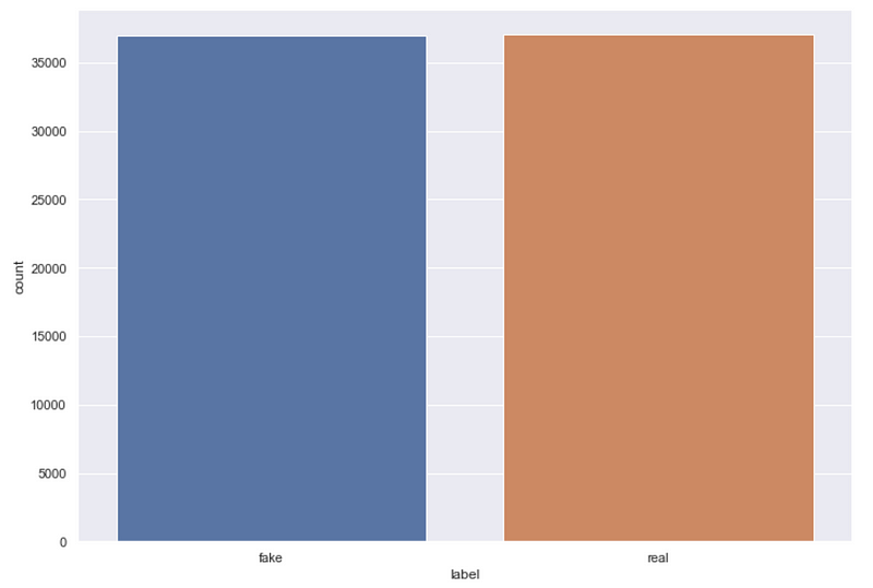

Distribution of Article Length (Word Count)

We can also examine the distribution of article lengths for the news articles using the code below, which creates a column that counts the word count of each article and displays the distribution of article lengths using Seaborn’s distplot function.

data['length'] = data['text'].apply(lambda x: len(x.split(' ')))
sns.distplot(data['length'])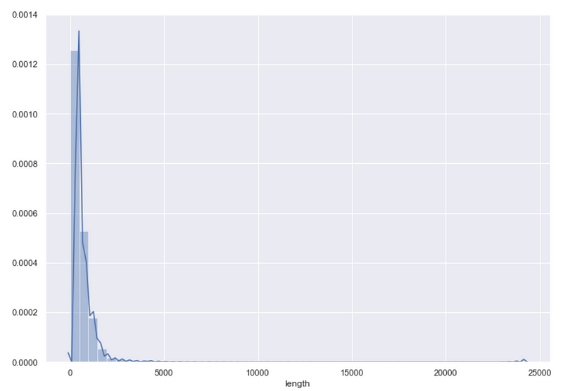

Taking a closer look at this distribution using the describe function from Pandas produces the following output.

data['length'].describe()

count    74012.000000
mean       549.869251
std        629.223073
min          1.000000
25%        235.000000
50%        404.000000
75%        672.000000
max      24234.000000
Name: length, dtype: float64

The average article length is about 550 words and the median article length is 404 words. The distribution is right-skewed with 75 percent of the articles having a word count under 672 words while the longest article is clearly an outlier with over 24,000 words. For the purpose of building a model, we could likely achieve satisfactory results by only using the first 500 or so words in each article to determine if it is fake news.

Data Preparation

Preprocessing the Text Data

The first step in preparing data for most natural language processing tasks is preprocessing the text data. For this task, I performed the following preprocessing steps in the preprocessor function defined below:

• Removing unwanted characters such as punctuation, HTML tags, and emoticons using regular expressions.
• Removing stop words (words that are extremely common in the English language and are generally not necessary for text classification purposes).
• Lemmatization, which is the process of reducing a word to its lemma or dictionary form. For example, the word run is the lemma for the words runs, ran, and running.

I used Python’s regex library to remove unwanted characters from the text data and Spacy’s medium-sized English language model (en_core_web_md) to perform stopword removal and lemmatization. In order to speed up the computation process for this expensive text-processing function, I made use of the parallel_apply function from Pandarallel, which parallelized the execution process across four cores.

import re 
from spacy.lang.en.stop_words import STOP_WORDS

nlp = en_core_web_md.load()

def preprocessor(text):
    text = re.sub('<[^>]*>', '', text)
    emoticons = re.findall('(?::|;|=)(?:-)?(?:\)|\(|D|P)', text)
    text = re.sub('[\W]+', ' ', text.lower()) + ''.join(emoticons).replace('-', '')
    doc = nlp(text)
    text = ' '.join([token.lemma_ for token in doc if token.text not in STOP_WORDS])
    return text

X = data['text'].parallel_apply(preprocessor)
y = data['label']

data_processed = pd.DataFrame({'title': data['title'], 'text': X, 'label': y})

Topic Modeling with Latent Dirichlet Allocation

After preprocessing the text data, I was able to use latent Dirichlet allocation (LDA) to compare the topics and most significant terms in real and fake news articles. LDA is an unsupervised topic modeling technique based on the following assumptions:

• Each document (in this case each news article) is a bag of words, meaning the order of words in the document is not taken into account when extracting topics.
• Each document has a distribution of topics and each topic is defined by a distribution of words.
• There are k topics across all documents. The parameter k is specified beforehand for the algorithm.
• The probability of a document containing words belonging to a specific topic can be modeled as a Dirichlet distribution.

In its simplest form, the LDA algorithm follows these steps for every document D in the collection of documents:

1. Distribute each of the k topics across the document D by assigning each word a topic according to the Dirichlet distribution.
2. For each word in D assume its topic is wrong but every other word is assigned the correct topic.
3. Assign this word a probability of belonging to each topic based on:
   – the topics in document D
   – how many times this word has been assigned to each topic across all documents.
4. Repeat steps 1–4 for all documents.

For a more detailed yet easily understandable overview of LDA, check out this page on Edwin Chen’s blog.

I used the LDA module from Scikit-learn to perform topic modeling and a useful Python library called pyLDAvis to create interactive visualizations of the topic models for both real and fake news. The necessary imports for this task are given below.

from sklearn.decomposition import LatentDirichletAllocation
from sklearn.feature_extraction.text import CountVectorizer
from sklearn.manifold import TSNE
from sklearn.pipeline import Pipeline
import pyLDAvis.sklearn

Real News

The code given below performs topic modeling on the preprocessed real news articles with ten different topics and then creates an interactive visualization that displays each topic in two-dimensional space using pyLDAvis.

real_news = data_processed[data_processed['label'] == 1]

num_topics = 10
num_features=5000

vectorizer = CountVectorizer(max_df=0.95, min_df=2, max_features=num_features, stop_words='english')
lda = LatentDirichletAllocation(n_components=num_topics,
                                max_iter=5, 
                                learning_method='online', 
                                learning_offset=50.,
                                random_state=0)

lda_pipeline = Pipeline([('vectorizer', vectorizer), ('lda', lda)])
lda_pipeline.fit(real_news['text'])

pyLDAvis.enable_notebook()
data_vectorized = vectorizer.fit_transform(data_processed['text'])
dash = pyLDAvis.sklearn.prepare(lda_pipeline.steps[1][1], data_vectorized, vectorizer, mds='tsne')

pyLDAvis.save_html(dash, 'real_news_lda.html')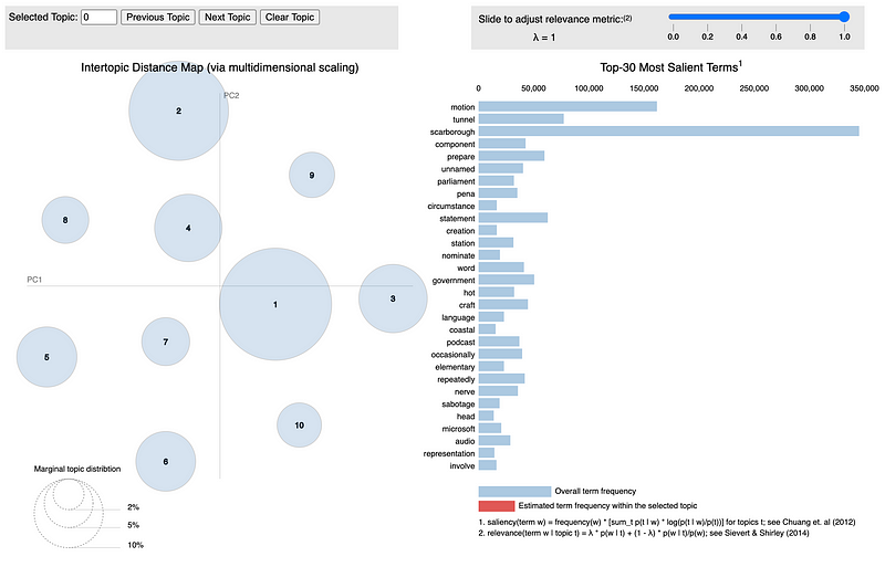

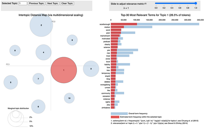
The visualization above allows the user to view the relative size of each of the ten extracted topics while displaying the most relevant terms for each topic. You can check out the full interactive visualization here.

Fake News

The code given below replicates the previous steps for the fake news articles to produce a similar interactive visualization.

fake_news = data_processed[data_processed['label'] == 0]

num_topics = 10
num_features=5000

vectorizer = CountVectorizer(max_df=0.95, min_df=2, max_features=num_features, stop_words='english')
lda = LatentDirichletAllocation(n_components=num_topics,
                                max_iter=5, 
                                learning_method='online', 
                                learning_offset=50.,
                                random_state=0)

lda_pipeline = Pipeline([('vectorizer', vectorizer), ('lda', lda)])
lda_pipeline.fit(fake_news['text'])

pyLDAvis.enable_notebook()
data_vectorized = vectorizer.fit_transform(data_processed['text'])
dash = pyLDAvis.sklearn.prepare(lda_pipeline.steps[1][1], data_vectorized, vectorizer, mds='tsne')

pyLDAvis.save_html(dash, 'fake_news_lda.html')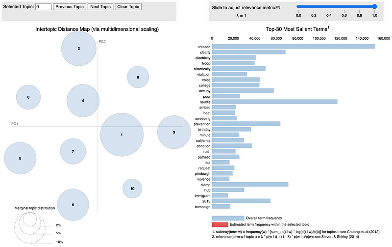

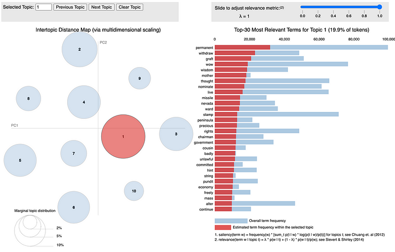
You can check out the full interactive visualization here. Based on the topic model visualizations for real and fake news, it is clear that fake news usually involves different topics when compared to real news. Based on the visualizations and some of the topic keywords such as treason, violation, pathetic, rush, and violence it seems that fake news generally covers more controversial topics such as alleged political scandals and conspiracy theories.

Defining and Training the Model

The deep learning model I designed for this task is a recurrent convolutional neural network model that consists of several different types of sequential operations and layers:

1. A tokenizer is used to transform each article into a vector of indexed words (tokens).
2. A word embedding layer that learns an embedding vector with m dimensions for each unique word and applies this embedding for the first n words in each news article, generating a m x n matrix.
3. 1D convolutional and max-pooling layers.
4. LSTM layers followed by dropout layers.
5. A final fully-connected layer.

These components are explained in greater detail below.

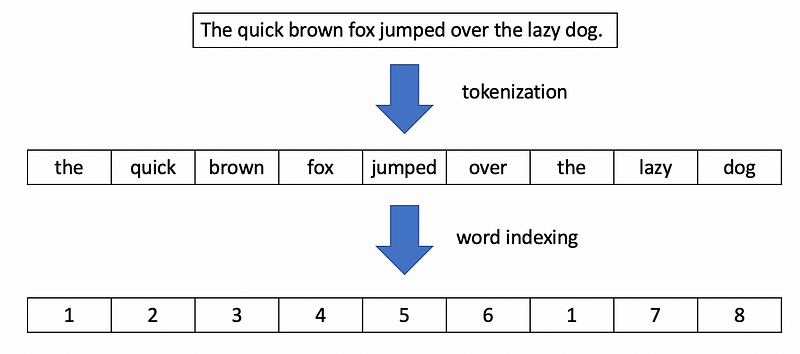
The Tokenizer

A tokenizer is used to split each news article into a vector of sequential words, which is later converted to a vector of integers by assigning a unique integer index to each word. The figure below demonstrates this process with a simple sentence.

Word Embedding Layers

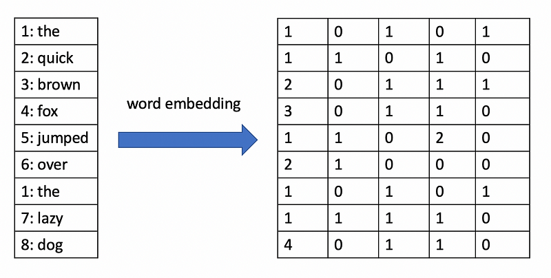
Word embeddings are learnable vector representations of words that represent the meaning of the words in relation to other words. Deep learning approaches can learn word embeddings from collections of text such that words with similar embedding vectors tend to have similar meanings or represent similar concepts.

1D Convolutional and Max-Pooling Layers

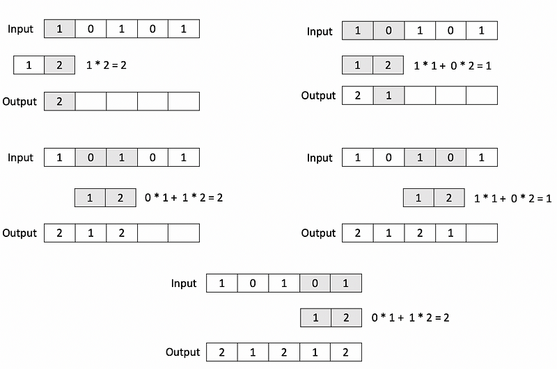
These components are the convolutional part of the recurrent convolutional neural network. If you have studied computer vision, you may be familiar with 2D convolutional and pooling layers that operate on image data. For text data, however, we need to use 1D convolutional and pooling layers. A 1D convolutional layer has a series of kernels, which are low-dimensional vectors that incrementally slide across the input vector as dot products are computed to produce the output vector. In the example below, a 1D convolutional operation with a kernel of size 2 is applied to an input vector with 5 elements.

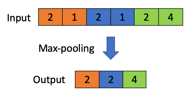
Like 1D convolutional layers, 1D max-pooling layers also operate on vectors but reduce the size of the input by selecting the maximum value from local regions in the input. In the example below, a max-pooling operation with a pool size of 2 is applied to a vector with 6 elements.

LSTMs

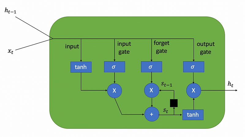
The LSTM (long short-term memory) units form the recurrent part of the recurrent convolutional neural network. LSTMs are often used for tasks involving sequence data such as time series forecasting and text classification. I won’t dive deeply into the mathematical background behind LSTMs because that topic is out of the scope of this article, but essentially an LSTM is a unit in a neural network capable of remembering essential information for long periods of time and forgetting information when it is no longer relevant (hence the name, long short-term memory). An LSTM unit consists of three gates:

• An input gate which receives the input values.
• A forget gate which decides how much of the past information acquired during training should be remembered.
• An output gate which produces the output values.

The ability of LSTMs to selectively remember information is useful in text classification problems such as fake news classification, since the information at the beginning of a news article may still be relevant to the content in the middle or towards the end of the article.

Fully-Connected Layer

The final part of this model is simply a fully-connected layer that you would find in a “vanilla” neural network. This layer receives the output from the last LSTM layer and computes a weighted sum of the vector values, applying a sigmoid activation to this sum to produce the final output — a value between 0 and 1 corresponding to the probability of an article being real news.

Putting it All Together

The class that I created below is designed for customizing and encapsulating a model with all of the components described above. This class represents a pipeline that can be fitted directly to preprocessed text data without having to perform steps such as tokenization and word indexing beforehand. The LSTM_Text_Classifier class extends the BaseEstimator and ClassifierMixin classes from Scikit-learn, allowing it to behave like a Scikit-learn estimator.

https://gist.github.com/AmolMavuduru/b8dbc121b8aec8319e244e0719fa72d0

Using this class, I created a model with the following components in the code below:

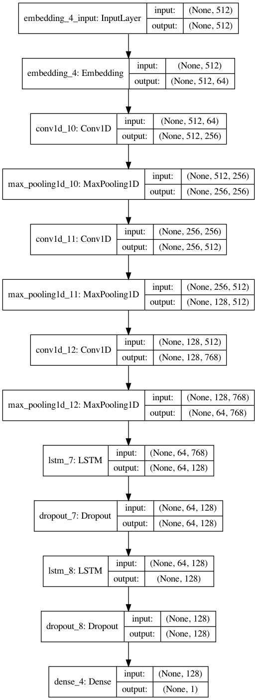
• A word embedding layer that learns a 64-dimensional embedding vector for each word and aggregates the vectors from the first 512 words of a news article to generate a 512 x 64 embedding matrix for each input article.
• Three convolutional layers with 128 convolutional filters and a kernel size of 5, each followed by a max-pooling layer.
• Two LSTM layers with 128 neurons, each followed by a dropout layer with a 10 percent dropout rate.
• A fully-connected layer at the end of the network with a sigmoid activation, outputting a single value ranging from 0 to 1 and indicating the probability of an article being real news.

lstm_classifier = LSTM_Text_Classifier(embedding_vector_length=64, max_seq_length=512, dropout=0.1, lstm_layers=[128, 128], batch_size=256, num_epochs=5, use_hash=False,
conv_params={'filters': 128, 
             'kernel_size': 5, 
             'pool_size': 2,
             'n_layers': 3})

The visualization below gives us a good idea of what the model architecture for this recurrent convolutional network looks like.

Training, Validation, and Testing Split

In order to evaluate the performance of this model effectively, it is necessary to split the data into separate training, validation, and testing sets. Based on the code below, 30 percent of the data is used for testing, and of the remaining 70 percent, 14 percent (20 percent of 70) is used for validation, and the remaining 56 percent is used for training.

from sklearn.model_selection import train_test_split
X_train, X_test, y_train, y_test = train_test_split(X, y, test_size=0.3, random_state=42)
X_train, X_valid, y_train, y_valid = train_test_split(X_train, y_train, test_size=0.2, random_state=42)

Model Training

After defining this complex model, I was able to train it on the training set while monitoring its performance on the validation set. The model was trained for three epochs and achieved its peak validation performance at the end second training epoch based on the code and output below.

lstm_classifier.fit(X_train, y_train, validation_data=(X_valid, y_valid))

Fitting Tokenizer...
Model: "sequential_4"
_________________________________________________________________
Layer (type)                 Output Shape              Param #   
=================================================================
embedding_4 (Embedding)      (None, 512, 64)           13169920  
_________________________________________________________________
conv1d_10 (Conv1D)           (None, 512, 256)          82176     
_________________________________________________________________
max_pooling1d_10 (MaxPooling (None, 256, 256)          0         
_________________________________________________________________
conv1d_11 (Conv1D)           (None, 256, 512)          655872    
_________________________________________________________________
max_pooling1d_11 (MaxPooling (None, 128, 512)          0         
_________________________________________________________________
conv1d_12 (Conv1D)           (None, 128, 768)          1966848   
_________________________________________________________________
max_pooling1d_12 (MaxPooling (None, 64, 768)           0         
_________________________________________________________________
lstm_7 (LSTM)                (None, 64, 128)           459264    
_________________________________________________________________
dropout_7 (Dropout)          (None, 64, 128)           0         
_________________________________________________________________
lstm_8 (LSTM)                (None, 128)               131584    
_________________________________________________________________
dropout_8 (Dropout)          (None, 128)               0         
_________________________________________________________________
dense_4 (Dense)              (None, 1)                 129       
=================================================================
Total params: 16,465,793
Trainable params: 16,465,793
Non-trainable params: 0
_________________________________________________________________
None
Fitting model...



Train on 41446 samples, validate on 10362 samples
Epoch 1/5
41446/41446 [==============================] - 43s 1ms/step - loss: 0.2858 - accuracy: 0.8648 - val_loss: 0.1433 - val_accuracy: 0.9505
Epoch 2/5
41446/41446 [==============================] - 42s 1ms/step - loss: 0.0806 - accuracy: 0.9715 - val_loss: 0.1192 - val_accuracy: 0.9543
Epoch 3/5
41446/41446 [==============================] - 43s 1ms/step - loss: 0.0381 - accuracy: 0.9881 - val_loss: 0.1470 - val_accuracy: 0.9527
Epoch 00003: early stopping

Validation Results

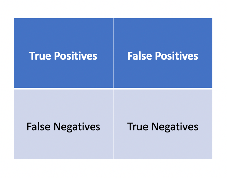
While accuracy is a useful metric for classification, it fails to tell us how the model is performing with respect to detecting each class. The code provided below computes the confusion matrix and classification report for the model’s predictions on the validation dataset to provide a better picture of the model’s performance. The confusion matrix provides classification statistics in the following format:

The classification report for each class provides the following additional metrics:

1. Precision — the number of times a class was correctly predicted divided by the total number of times the model predicted this class.
2. Recall — the number of times a class was correctly predicted divided by the total number of samples with that class label in the testing data.
3. F1-Score — the harmonic mean of precision and recall.

lstm_classifier.load_model('best_model')

from sklearn.metrics import confusion_matrix, classification_report

y_pred = lstm_classifier.predict_classes(X_valid)
print(confusion_matrix(y_valid, y_pred))
print(classification_report(y_valid, y_pred, digits=4))

[[4910  204]
 [ 271 4977]]
              precision    recall  f1-score   support

           0     0.9477    0.9601    0.9539      5114
           1     0.9606    0.9484    0.9545      5248

    accuracy                         0.9542     10362
   macro avg     0.9542    0.9542    0.9542     10362
weighted avg     0.9542    0.9542    0.9542     10362

Based on the results above, we can clearly see that the model is nearly as good at detecting fake news correctly as it is at detecting real news correctly and achieved an overall accuracy of 95.42 percent on the validation data, which is pretty impressive. According to the confusion matrix, only 271 articles were misclassified as fake news and only 204 articles were misclassified as real news.

Testing Results

While the validation results can give us some indication of the model’s performance on unseen data, it is the testing set, which has not been touched at all during the model training process which provides the best objective and statistically correct measure of the model’s performance. The code below produces a classification report for the testing set.

from sklearn.metrics import accuracy_score

y_pred_test = lstm_classifier.predict_classes(X_test)
print(classification_report(y_test, y_pred_test))

               precision    recall  f1-score   support

           0       0.94      0.95      0.95     11143
           1       0.95      0.94      0.95     11061

    accuracy                           0.95     22204
   macro avg       0.95      0.95      0.95     22204
weighted avg       0.95      0.95      0.95     22204

Based on the output above, the model achieved a similar level of performance on the testing set compared to its performance on the validation set. The model classified news articles in the testing set with an accuracy of 95 percent. Compared to the study in which humans were able to detect fake news only 70 percent of the time, these results are promising and demonstrate that a trained neural network could potentially do a better job at filtering out fake news than a human reader.

Conclusions

• Based on the LDA visualizations, we can see that there is a different distribution of topics and associated keywords for real and fake news.
• The recurrent convolutional neural network used in this project was able to distinguish between real and fake news articles with 95 percent accuracy on the testing data, which suggest that neural networks can potentially detect fake news better than human readers.

Feel free to check out the Jupyter notebook with the code for this article on GitHub.

Sources

1. V. Pérez-Rosas, B. Kleinberg, A. Lefevre, R. Mihalcea, Automatic Detection of Fake News, (2018), arXiv.org
2. A. Bharadwaj, B. Ashar, P. Barbhaya, R. Bhatia, Z. Shaikh, Source-Based Fake News Classification using Machine Learning, (2020), International Journal of Innovative Research in Science, Engineering and Technology